Download
1 / 40
400 likes | 571 Vues
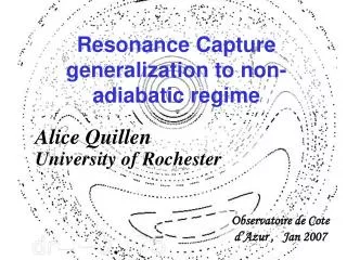
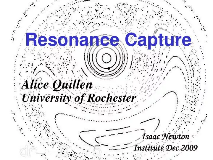
Resonance Capture. Alice Quillen University of Rochester. Isaac Newton Institute Dec 2009. This Talk. Resonance Capture – extension to non-adiabatic regime Astrophysical settings: Dust spiraling inward via radiation forces (PR drag) when collisions are not important

E N D
Resonance Capture Alice Quillen University of Rochester Isaac Newton Institute Dec 2009
This Talk • Resonance Capture – extension to non-adiabatic regime • Astrophysical settings: • Dust spiraling inward via radiation forces (PR drag) when collisions are not important • Neptune or exoplanet or satellite migrating outward • Jupiter or exoplanet or satellite migrating inward • Multiple exoplanets drifting into resonance Resonances are thin, but sticky (random drift leads to capture, in some cases increased stability)
Example of Resonance Capture Production of Star Grazing and Star-Impacting Planetesimals via Planetary Orbital MigrationQuillen & Holman 2000, but also see Quillen 2002 on the Hyades metallicity scatter Eject Impact FEB
Simple Hamiltonian systems Harmonic oscillator I θ p q Stable fixed point Libration Oscillation Pendulum p Separatrix
Resonant angle In the frame rotating with the planet Librating resonant angle in resonance Oscillating resonant angle outside resonance Image by Marc Kuchner
Drifting Pendulum and distance to resonance Fixed points at Canonical transformation with zero p 0- bsets distance to resonance A drifting system can be modeled with time varying b or db/dt setting drift rate
Dimensional Analysis on the Pendulum • H units cm2 s-2 • Action variable p cm2 s-1 (H=Iω) and ω with 1/s • a cm-2 • b s-1 • Drift rate db/dt s-2 • ε cm2 s-2 Ignoring the distance from resonance we only have two parameters, a,ε • Only one way to combine to get momentum • Only one way to combine to get time
Resonant width and Libration period • Resonant width solve H(p,θ) =0 for maximum p. Distance to separatrix • Libration timescale, expand about fixed point Libration period p note similarity between these expressions and those derived via dimensional analysis
resonant angle fixed - Capture Escape Behavior of a drifting resonant system • We would like to know the capture probability as a function of: • initial conditions • migration or drift rate • resonance properties eccentricity jump eccentricity increase
Adiabatic Invariants • If motion is slow one can average over phase angle • Action variable is conserved • Volume in phase space is conserved as long as drifting harmonic oscillator
Adiabatic Capture Theoryfor Integrable Drifting Resonances Theory introduced by Yoder and Henrard, special treatment of separatrix that has an infinite period Applied to mean motion resonances by Borderies and Goldreich, Malhotra, Peale …
Adiabatic limit for drifting pendulum • Drift rate should be slow • Time to drift the resonant width should be much longer than libration timescale Via dimensional analysis. Units of db/dt are s-2. Our only unit of time is • We are in the adiabatic limit if Note there is no capture if dε/dt=0 as the volume in the resonance does not grow
Keplerian Hamiltonian • Unperturbed, in the plane • Poincaré coordinates • Hamiltonian only depends on Λ. Everything is conserved except λ which advances with λ mean longitude -γ=ϖ longitude of perihelion
Expand Near Resonance Must keep distance to resonance (b) and take expansion to at least second order in momentum otherwise our Hamiltonian won’t look like a pendulum and so won’t be able to differentiate between libration and oscillation Note: we have the first part of our pendulum Hamiltonian
Our perturbation • R, The disturbing function • μ ratio of planet mass to stellar mass • ap np Planet semi-major axis and mean motion • Wm Laplace coefficient – comes from integral of GM*mp/|r-rp| over orbit • Radius r will be expanded in terms of eccentricity giving us terms like Γ1/2 cos(jλ – (j-1)λp – ϖ) • Note: we are getting cosine terms like our pendulum
Full Hamiltonian • Putting together H0 (unperturbed but expanded near resonance) and R (planetary perturbation) • We ignore all cosine terms with rapidly varying angles We get something that looks our pendulum Hamiltonian • Examples of expansion near resonance • Murray & Dermott, Solar System Dynamics, section 8.8 • Holman, M. & Murray, N. 1996 AJ, 112, 1278 • Quillen 2006, MNRAS, 365, 1367
Canonical Transformation and reducing the dimension New Hamiltonian only depends on one coordinate φ, so all action variables are conserved except P1 generating function
Andoyer Hamiltonian(see appendix C of book by Ferraz-Mello) • k is order of resonance or power of eccentricity in low eccentricity expansion • If p is large then we can think of as a resonance width, and p as varying about the initial value • The resonance will not grow much during drift unlikely to capture Low eccentricity formulism is pretty good for resonance capture prediction
k=1 Structure of Resonance • Radius on plot is ~ eccentricity • When b~0 there are NO circular orbits • Capture means lifting into one of the islands where the angle becomes fixed (does not circulate) • Capture in only one direction of drift increasing b
Computing probability involves computing volumes when separatrix appears starting with eccentricity below critical value 100% capture starting with eccentricity above critical value Images from Murray and Dermott’s Book Solar System Dynamics
Resonance Capture in the Adiabatic Limit • Application to tidally drifting satellite systems by Borderies, Malhotra, Peale, Dermott, based on analytical studies of general Hamiltonian systems by Henrard and Yoder. • Capture probabilities are predicted as a function of resonance order and coefficients via integration of volume • Capture probability depends on initial particle eccentricity. -- Below a critical eccentricity capture is ensured.
Limitations of Adiabatic theory • At fast drift rates resonances can fail to capture -- the non-adiabatic regime. • Subterms in resonances can cause chaotic motion φ e Λ,Γ temporary capture in a chaotic system
Chaotic Tidal Evolution of Uranian Satellites Tittemore & Wisdom Tittemore & Wisdom 1990
Dimensional analysis on the Andoyer Hamiltonian • We only have two important parameters if we ignore distance to resonance • a dimension cm-2 • ε dimension cm2-k s-2-k/2 • Only one way to form a timescale and one way to make a momentum sizescale. • The square of the timescale will tell us if we are in the adiabatic limit • The momentum sizescale will tell us if we are near the resonance (and set critical eccentricity ensuring capture in adiabatic limit)
Rescaling This factor sets dependence on initial eccentricity This factor sets dependence on drift rate All k-order resonances now look the same opportunity to develop a general framework
Rescaling Drift rates have units t-2 First order resonances have critical drift rates that scale with planet mass to the power of -4/3. Second order to the power of -2. Confirming and going beyond previous theory by Friedland and numerical work by Ida, Wyatt, Chiang..
Probability of Capture log drift rate Numerical Integration of rescaled systems Capture probability as a function of drift rate and initial eccentricity First order resonances At low initial eccentricity the transition is very sharp First order Critical drift rate– above this capture is not possible high initial eccentricity Transition between “low” initial eccentricity and “high” initial eccentric is set by the critical eccentricity below which capture is ensured in the adiabatic limit (depends on rescaling of momentum). See Alex Mustil on sensitivity to initial conditions.
Second order resonances Probability of Capture log drift rate Capture probability as a function of initial eccentricity and drift rate High initial particle eccentricity allows capture at faster drift rates low initial eccentricity
Probability of Capture drift rate Sensitivity to Initial Eccentricity At high eccentricity initial the resonance doesn’t grow much but libration takes place on a faster timescale Weak resonances can capture at low probability in high eccentricity regime
Adding additional terms • If we include additional terms we cannot reduce the problem by a dimension • In the plane a 4D phase space • This system is not necessarily integrable
Role of corotation resonance in preventing capture drift separation set by secular precession rate • Above in rescaled units • There is another libration timescale in the problem set by • Corotation resonance cannot grow during drift so it cannot capture. But it can be fast enough to prevent capture. corotation resonance proportional to planet eccentricity
drift separation set by secular precession When there are two resonant terms Capture is prevented by corotation resonance depends on planet eccentricity escape Capture is prevented by a high drift rate log ε (corotation strength) capture log drift rate
Comment on Temporary Capture • x Tittemore & Wisdom 1990 ~ Slow evolution in one degree of freedom pulls other out of resonance?
Limits Critical drift rates defining the adiabatic limit for each resonance can be computed from resonance strengths.
Other uses for dimensional analysis • If resonance fails to capture, there is jump in eccentricity. (e.g. eccentricity increases caused by divergent migrating systems when they go through resonance). Can be predicted dimensionally or using toy model and rescaling. • Resonant width at low e can be estimated by estimating the range of b where the resonance is important. Jack Wisdom’s μ2/3 for first order resonances. • Perturbations required to push a particle out of resonance can be estimated
Trends • Higher order (and weaker) resonances require slower drift rates for capture to take place. Dependence on planet mass is stronger for second order resonances. • If the resonance is second order, then a higher initial particle eccentricity will allow capture at faster drift rates – but not at high probability. • If the planet is eccentric the corotation resonance can prevent capture • Resonance subterm separation (set by the secular precession frequencies) does affect the capture probabilities – mostly at low drift rates – the probability contours are skewed.
Applications to Neptune’s migration Few objects captured in 2:1 and many objects interior to 2:1 suggesting that capture was inefficient • Neptune’s eccentricity is ~ high enough to prevent capture of TwoTinos. 2:1 resonance is weak because of indirect terms, but corotation term not necessarily weak. • Critical drift rate predicted is more or less consistent with previous numerical work. image from wiki
Lynnette Cook’s graphic for 55Cnc Application to multiple planet systems This work has not yet been extended to do 2 massive bodies, but could be. Resonances look the same but coefficients must be recomputed and role of multiple subterms considered. A migrating extrasolar planet can easily be captured into the 2:1 resonance with another large planet but must be moving fairly slowly to capture into the 3:1 resonance. ~Consistent with timescales chosen by Kley for hydro simulations. Super earth’s require slow drift to capture each other.
Final Comments • Formalism is general – if you look up resonance coefficients, critical drift rates for non adiabatic limit can be estimated for any resonance : (Quillen 2006 MNRAS 365, 1367) See my website for errata! There is a new one not in there yet found by Alex Mustill • This “theory” has not been checked numerically. Values for critical drift rate predicted via rescaling have not been verified to factors of a few. • We have progress in predicting the probability of resonance capture, however we lack good theory for predicting lifetimes • No understanding of k=>4 • Evolution during temporary capture can be complex • Evolution following capture can be complex • Extension to 2 massive bodies not yet done