Download
1 / 66
690 likes | 841 Vues
CS6670: Computer Vision. Noah Snavely. Lecture 2: Edge detection and resampling. From Sandlot Science. Administrivia. New room starting Thursday: HLS B11. Administrivia. Assignment 1 (feature detection and matching) will be out Thursday Turning via CMS: https://cms.csuglab.cornell.edu/

E N D
CS6670: Computer Vision Noah Snavely Lecture 2: Edge detection and resampling From Sandlot Science
Administrivia • New room starting Thursday: HLS B11
Administrivia • Assignment 1 (feature detection and matching) will be out Thursday • Turning via CMS: https://cms.csuglab.cornell.edu/ • Mailing list: please let me know if you aren’t on it
Reading • Szeliski: 3.4.1, 3.4.2
Last time: Cross-correlation Let be the image, be the kernel (of size 2k+1 x 2k+1), and be the output image This is called a cross-correlation operation:
Last time: Convolution • Same as cross-correlation, except that the kernel is “flipped” (horizontally and vertically) This is called a convolution operation:
0 0 0 0 1 0 0 0 0 Linear filters: examples = * Original Identical image Source: D. Lowe
0 0 0 1 0 0 0 0 0 Linear filters: examples = * Original Shifted left By 1 pixel Source: D. Lowe
1 1 1 1 1 1 1 1 1 Linear filters: examples = * Original Blur (with a mean filter) Source: D. Lowe
0 1 0 1 1 0 1 0 1 2 0 1 0 1 1 0 0 1 Linear filters: examples - = * Sharpening filter (accentuates edges) Original Source: D. Lowe
Image noise Original image Gaussian noise Salt and pepper noise (each pixel has some chance of being switched to zero or one) http://theory.uchicago.edu/~ejm/pix/20d/tests/noise/index.html
Gaussian noise = 1 pixel = 2 pixels = 5 pixels Smoothing with larger standard deviations suppresses noise, but also blurs the image
Salt & pepper noise – Gaussian blur p = 10% = 1 pixel = 2 pixels = 5 pixels • What’s wrong with the results?
Alternative idea: Median filtering • A median filter operates over a window by selecting the median intensity in the window • Is median filtering linear? Source: K. Grauman
Median filter • What advantage does median filtering have over Gaussian filtering? Source: K. Grauman
Salt & pepper noise – median filtering p = 10% = 1 pixel = 2 pixels = 5 pixels 3x3 window 5x5 window 7x7 window
Edge detection • Convert a 2D image into a set of curves • Extracts salient features of the scene • More compact than pixels TexPoint fonts used in EMF. Read the TexPoint manual before you delete this box.: AAA
Origin of Edges Edges are caused by a variety of factors surface normal discontinuity depth discontinuity surface color discontinuity illumination discontinuity
intensity function(along horizontal scanline) first derivative edges correspond toextrema of derivative Characterizing edges • An edge is a place of rapid change in the image intensity function image Source: L. Lazebnik
Image derivatives • How can we differentiate a digital image F[x,y]? • Option 1: reconstruct a continuous image, f, then compute the derivative • Option 2: take discrete derivative (finite difference) How would you implement this as a linear filter? : : Source: S. Seitz
Image gradient • The gradient of an image: The gradient points in the direction of most rapid increase in intensity • The edge strength is given by the gradient magnitude: • The gradient direction is given by: • how does this relate to the direction of the edge? Source: Steve Seitz
Image gradient Source: L. Lazebnik
Effects of noise Noisy input image Where is the edge? Source: S. Seitz
h f * h Solution: smooth first f To find edges, look for peaks in Source: S. Seitz
f Associative property of convolution • Differentiation is convolution, and convolution is associative: • This saves us one operation: Source: S. Seitz
2D edge detection filters derivative of Gaussian (x) Gaussian
Derivative of Gaussian filter y-direction x-direction
The Sobel operator Common approximation of derivative of Gaussian • The standard defn. of the Sobel operator omits the 1/8 term • doesn’t make a difference for edge detection • the 1/8 term is needed to get the right gradient value
Sobel operator: example Source: Wikipedia
Example • original image (Lena)
Finding edges gradient magnitude
Finding edges where is the edge? thresholding
Non-maximum supression • Check if pixel is local maximum along gradient direction • requires interpolating pixels p and r
Finding edges thresholding
Finding edges thinning (non-maximum suppression)
Canny edge detector MATLAB: edge(image,‘canny’) • Filter image with derivative of Gaussian • Find magnitude and orientation of gradient • Non-maximum suppression • Linking and thresholding (hysteresis): • Define two thresholds: low and high • Use the high threshold to start edge curves and the low threshold to continue them Source: D. Lowe, L. Fei-Fei
Canny edge detector • Still one of the most widely used edge detectors in computer vision • Depends on several parameters: J. Canny, A Computational Approach To Edge Detection, IEEE Trans. Pattern Analysis and Machine Intelligence, 8:679-714, 1986. : width of the Gaussian blur high threshold low threshold
Canny edge detector original Canny with Canny with • The choice of depends on desired behavior • large detects “large-scale” edges • small detects fine edges Source: S. Seitz
first derivative peaks Scale space (Witkin 83) • Properties of scale space (w/ Gaussian smoothing) • edge position may shift with increasing scale () • two edges may merge with increasing scale • an edge may not split into two with increasing scale larger Gaussian filtered signal
Image Scaling This image is too big to fit on the screen. How can we generate a half-sized version? Source: S. Seitz
Image sub-sampling 1/8 1/4 • Throw away every other row and column to create a 1/2 size image • - called image sub-sampling Source: S. Seitz
Image sub-sampling 1/2 1/4 (2x zoom) 1/8 (4x zoom) Why does this look so crufty? Source: S. Seitz
Image sub-sampling Source: F. Durand
Even worse for synthetic images Source: L. Zhang
Aliasing • Occurs when your sampling rate is not high enough to capture the amount of detail in your image • Can give you the wrong signal/image—an alias • To do sampling right, need to understand the structure of your signal/image • Enter Monsieur Fourier… • To avoid aliasing: • sampling rate ≥ 2 * max frequency in the image • said another way: ≥ two samples per cycle • This minimum sampling rate is called the Nyquist rate Source: L. Zhang
Wagon-wheel effect (See http://www.michaelbach.de/ot/mot_wagonWheel/index.html) Source: L. Zhang
Gaussian pre-filtering G 1/8 G 1/4 Gaussian 1/2 • Solution: filter the image, then subsample Source: S. Seitz
Subsampling with Gaussian pre-filtering Gaussian 1/2 G 1/4 G 1/8 • Solution: filter the image, then subsample Source: S. Seitz