Download
1 / 17
180 likes | 391 Vues
Mid Term 2. Hough Transform Line, circle fitting Generalized Hough transform Interest point, corner detectors Pixel based optical flow Token based optical flow Global motion Shape from motion Geometry of a stereo camera pair Stereopsis Fundamental matrix (estimation)

E N D
Mid Term 2 • Hough Transform • Line, circle fitting • Generalized Hough transform • Interest point, corner detectors • Pixel based optical flow • Token based optical flow • Global motion • Shape from motion • Geometry of a stereo camera pair • Stereopsis • Fundamental matrix (estimation) • Graph based image segmentation Alper Yilmaz, Fall 2004 UCF
Hough Transform Interest point, corner detectors Pixel based optical flow Token based optical flow Global motion Alper Yilmaz, Fall 2004 UCF
Hough Transform • Line fitting • 2D accumulator array A. Fix compute . • Increment (,) entry of A • Circle fitting • 3D accumulator array A. Fix x0, y0 compute r. • Increment (x0,y0,r) entry of A • Practical circle fitting • Compute gradient direction at an edge point () • Fix r compute • Increment (x0,y0,r) entry of A Alper Yilmaz, Fall 2004 UCF
1 r1, r2, r3 … 2 r14, r21, r23 … 3 r41, r42, r33 … 4 r10, r12, r13 … Generalized Hough Transform • For shapes with no analytical expression • Requires learning of shape • For each edge compute direction and distance r from centroid • Construct a table indexed by (r-table) • Shape fitting (detecting) • Construct 2D accumulator array for (x0,y0) • Compute gradient direction for each edge point • Go to corresponding row of r-table • Compute possible x0 and y0 from (,r) pair • Increment accumulator array Alper Yilmaz, Fall 2004 UCF
Interest Points and Corner • High texture variation around a pixel • T-joints, cross joints etc. • Movarec’s interest operator • Select 12x12 neighborhood around a pixel • Compute intensity variation v in overlapping 4x4 neighborhoods • If v for central 4x4 is equal or higher to v all other 4x4, mark pixel as interest point Alper Yilmaz, Fall 2004 UCF
Harris Corner detector • Smooth image (gaussian filter) • Compute image derivatives Ix and Iy • Smooth image gradients (gaussian filter) • Construct gradient matrix in a neighborhood • Find eigenvalues of M • Save smallest eigenvalue in a corner strength array A • Perform non-maximum to A and apply threshold to mark corners Alper Yilmaz, Fall 2004 UCF
d . Optical Flow • Brightness constancy • For given Ix, Iy and It there are a set of (u,v) pairs Taylor series expansion v Normal flow (can be computed) Parallel flow (can NOT be computed) p u Alper Yilmaz, Fall 2004 UCF
Optical Flow • Horn & Schunck (1981) • Regularization of optical flow (defines 2 energy terms) • Brightness constraint energy • Smoothness energy • Minimize iteratively • Schunk (1989) • Neighboring pixels move with same motion • Form intersecting lines in (u,v) space • Biggest cluster of intersection is the optical flow Alper Yilmaz, Fall 2004 UCF
Optical Flow • Lucas & Kanade (1981) • Least squares method. Minimize • Take derivatives wrt. u and v equal it to 0. • 2 unknowns 2 equations (Lecture 14 slides 26-28) • Compute unknowns using least squares. Alper Yilmaz, Fall 2004 UCF
Optical Flow • Optical methods work only for small motion. • If object moves faster, the brightness changes rapidly, derivative masks fail to estimate spatiotemporal derivatives. • Gaussian pyramids can be used to compute large optical flow vectors. Alper Yilmaz, Fall 2004 UCF
Block Based Optical Flow • First approach • Find tokens in 1st image • Search similar tokens in 2nd image using correlation methods • Second approach • Find tokens (corners etc.) in both images • Find correspondence between tokens by enforcing constraints, such as, maximum speed, common motion, minimum velocity, consistent match Alper Yilmaz, Fall 2004 UCF
Block Based Optical FlowFirst Approach • Select a patch P image at time t • Search for P at frame t+1 in a larger neighborhood • Compute similarity between original patch and search patch • Construct a correlation surface • Select maximum Alper Yilmaz, Fall 2004 UCF
Block Based Optical FlowIssues With Correlation • Patch Size • Search Area • How many peaks • Computationally expensive • Same operations in Fourier domain takes less time • Take FFT of image patch and search area • Multiply Fourier coefficients to construct corr. surface • Find maximum • Should use pyramids here too for large displacements Alper Yilmaz, Fall 2004 UCF
Block Based Optical FlowSecond Approach • Find initial correspondences using correlation • Compute costs wij for each pair of points ai, bj • Construct a bipartite graph based on computed costs • Prune all edges having weights exceeding certain threshold • Define cost matrix • Find the minimum matching of constructed graph. • Hungarian Algorithm • Greedy search Alper Yilmaz, Fall 2004 UCF
Global Motion (Anandan’s Approach) • Common motion observed by most of the pixels in the frame • Reasons are camera motion or motion of rigid scene • Uses brightness constraint • Common motion model is affine (among others) • Affine can handle translation, rotation, shear, scaling • Minimize energy function • Unknowns are a1…a4,b1,b2 • Take derivative make it equal to zero Alper Yilmaz, Fall 2004 UCF
Global Motion (Anandan’s Approach) A B Alper Yilmaz, Fall 2004 UCF
(x’’,y’’) (x’,y’) (x,y) image at time t image at time t+1 intermediate iteration Iterative Update of Affine Parameters Alper Yilmaz, Fall 2004 UCF