Download
1 / 19
190 likes | 412 Vues
Orbit distortion and correction. David Kelliher ASTeC /STFC/RAL EMMA commissioning workshop, 2-4 December 2009. Contents. Orbit distortion Finding closed orbit “Target” orbit Response matrix calculation Orbit correction Number of monitors. Correction issues in EMMA.

E N D
Orbit distortion and correction David Kelliher ASTeC/STFC/RAL EMMA commissioning workshop, 2-4 December 2009
Contents • Orbit distortion • Finding closed orbit • “Target” orbit • Response matrix calculation • Orbit correction • Number of monitors
Correction issues in EMMA • No “Reference orbit” as in a synchrotron • Change of phase with energy – correction at one energy may not work at another • Decoherence • Horizontal distortion fixed by shifting the quadrupoles, vertical distortion fixed using corrector magnets
Ideal and distorted orbits Traditional method • Measure distortion w.r.t ideal orbit. • Aim of correction – bring distorted orbit back to ideal orbit • This approach makes sense in a synchrotron FFAG method • Ideal orbit is not known • Aim of correction – • Increase the symmetry of orbit (avoid resonances) • Increase the physical aperture
Closed orbit distortion study • Assume beam has already made it around the ring a few turns • Assume injection onto the distorted closed orbit achieved. • Consider horizontal misalignments only
Finding the closed orbit • Use position data recorded at each BPM. Assume no horizontal angle available. • Minimise variation of turn-by-turn data at each BPM by scanning injected x,x’ • Python script find_closed_orbit_bpmuses brute force method • Includes BPM noise and systematic error
Closed orbit distortion over energy range Maximum c.o.d - average of 100 error patterns . Error bar represents 1 sigma. Input misalignment distribution with 50 micron sigma and 2 sigma cut off. 100 error patterns. 0.1 MeV steps from 10-20 MeV.
Target orbit Distorted closed orbit @ 17.5 MeV. Input misalignment distribution with 50 micron sigma and 2 sigma cut off.
Correction to target orbit Distorted and corrected closed orbit @ 17.5 MeV. Input misalignment distribution with 50 micron sigma and 2 sigma cut off. All quadrupoles moved, perfect response matrix assumed
Response matrix calculation (1) • xBPM=A.shift • Response matrix A found by moving each quadrupole by a set amount. • Find new closed orbit. Decoherence should help reduce effect of betatron oscillations. • Change in BPM readings noted. Return quadrupole to nominal position.
Response matrix calculation (2) • Need to see the BPM signal due to magnet shift. Assume 50 micron noise on BPMs • Resolution of magnet move (3 microns) should be considered • Averaging over more turns will help 42 BPMs with 50 micron noise. 1 turn only.
Orbit Correction by least squares minimisation • Assuming perfect BPMs • Distortion to correct = Deviation from average BPM readings • Minimise |A.x – b| using Numpy linear algebra routine for least square minisation
Orbit Correction by least squares minimisation microns All 84 monitors available Input misalignment distribution with 50 micron sigma and 2 sigma cut off. 1 error pattern.
Number of monitors • Calculate orbit correction with 84, 42, 28, 21, 17, 14 monitors. Monitors are spread evenly around the ring. • Resulting distortion calculated at all 84 monitors
Orbit Correction by SVD • SVD method, decompose A = U.w.VT • Find inverse Ainv = V.winv.UT • Numpy routine numpy.linalg.svd(A) • Construct inverse singular values from diagonal maxtrix w, eliminating those below some threshold.
Singular values All 84 monitors available Input misalignment distribution with 50 micron sigma and 2 sigma cut off. 1 error pattern.
Eliminating low singular values All 84 monitors available Input misalignment distribution with 50 micron sigma and 2 sigma cut off. 1 error pattern.