Download
1 / 29
290 likes | 516 Vues
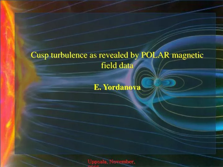
Cusp turbulence as revealed by POLAR magnetic field data E. Yordanova. Uppsala, November, 2005. Outline. Cusp Models of turbulence Multifractal structure of cusp turbulence Anisotropy in the cusp. Uppsala, November, 2005. depressed and irregular magnetic magnetic field

E N D
Cusp turbulence as revealed by POLAR magnetic field data E. Yordanova Uppsala, November, 2005
Outline • Cusp • Models of turbulence • Multifractal structure of cusp turbulence • Anisotropy in the cusp Uppsala, November, 2005
depressed and irregular magnetic magnetic field • magnetosheath plasma /high density and low energy/ • plasma ofionospheric origin Cusp • the direction of IMF • the tilt of the magnetic dipole • the solar wind dynamic pressure Uppsala, November, 2005
Turbulent magnetic field in the cusp POLARmission f < 10-2 Hz f < 102-103 Hz Uppsala, November, 2005
Examples of power spectra of the magnetic field fluctuations, measured in the cusp (POLAR satellite) By110497_1 B091096_5 Uppsala, November, 2005
Magnetospheric cusp magnetic field (POLAR satellite) cusps ramps spirals The singularity strength: Singularity spectrum D(h) • the statistical distribution of the singularity exponents h. Hölder exponenth(x0) - a measure of the regularity of the function g at the point x0 - a humped shape (hmin- strongest singularity; hmax –weakest singularity) Uppsala, November, 2005
Wavelet Transform (WT)A tool for detecting the singularities a - scale, b – translation or dilation, * - conjugated transforming function Wavelet Transform Modulus Maxima Method (WTMM) Mallat and Zong(1992) a maximum in the modulus of the wavelet transform coefficients Singularities ‘any point (x0,a0) of the space-scale half-plane which corresponds to the local maximum of the modulus of considered as a function of x’ Modulus maximum of WT the curve, connecting the modulus maxima Maxima line a power law fit of the wavelet coefficients along the maxima line Singularity exponents Uppsala, November, 2005
Kolmogorov phenomenology (1941) Energy injection Richardson cascade Inertial range . . . . . . . . . . . . . . . . Dissipation range Self-similarityin the inertial range Localness in the interaction Uppsala, November, 2005
P model (Meneveau and Sreenivasan ‘87) Energy injection Inertial range . . . . . . . . . . . . . . . . Dissipation range Uppsala, November, 2005
Structure functionsof a measured fluctuating parameter g(x): !fundamental quantity in classical theory of turbulence! Singularity spectrum(Parisi and Frisch,1985) Legendre transform D(h) - statistical distribution of the singularity exponentsh Calculation of the scaling properties of turbulence Uppsala, November, 2005
WTMM Wavelet based partition function (Muzy, Bacry, Arneodo, 1991): L(a) -a set of all the maxima lines lexisting at a scale a; bl(a) -the position, at a, of the maximum belonging to the line l Scaling law of the partition function along the maxima line: Singularity spectrum D(h) of the WTMM function (q): Relation between q and q l={bl(a), a}is pointing towards a pointbl(0)(when agoes to 0) which corresponds to a singularity of g Uppsala, November, 2005
- scaling exponents for the Kolmogorov-like cascade: P-model - scaling exponents for the Kraichnan-like cascade: Extended structure function models (Tu et al. 1996, Marsch and Tu 1997) Uppsala, November, 2005
The problem MF fluctuations – singular behavior Set of locations and strength of the singularities – singularity spectrum Method: WTMM Constructing partition functions – sums of the WT located in the modulus maxima (define the singularity) Uppsala, November, 2005
WTMM partition functions WTMM partition function exponents Fractional brownian signal Singularity spectrum Muzy, Bacry & Arneodo(1994) Uppsala, November, 2005
WTMM partition functions WTMM partition function exponents Devil’s staircase signal Singularity spectrum Muzy, Bacry & Arneodo(1994) Uppsala, November, 2005
partition function exponents (power law fit of wavelet coefficients along maxima line) Through numerical differentiation of the exponents curve singularity spectrum is derived (parabolic shape, typical for the non-linear systems) Non-linear behavior Mean square deviation between numerical and theoretical spectra Least-square fit of models of turbulence Comparison with models of turbulence Uppsala, November, 2005
Data sampling frequency - 8.333 Hz Probability distribution functions for different time delays Uppsala, November, 2005
Results for 9 Oct 1996 case p- model turbulence Bz > 0 Kolmogorov – like turbulence Bz < 0 Uppsala, November, 2005
Results for 11 Apr 1997 case Kolmogorov – like turbulence p - model turbulence Bx > 0 By < 0 Bz > 0 Uppsala, November, 2005
HYDRA / POLAR Uppsala, November, 2005
1. Conclusions about the magnetic field intensity IMF Bz > 0 – p – model (fluid, fully developed) IMF Bz < 0 - Kolmogorov- like (fluid, non fully developed) Uppsala, June, 2005
SPC Bz north antisun Bxy dusk B56 Anisotropy features of the magnetic field B~90 nT B~10 nT (Bxy, Bz, B56) (B1, B2, B0) Uppsala, November, 2005
~ 1.62 ~ 2.41 Power spectra in parallel and perpendicular directions f -5/3 ~ 1.21 ~ 5 ~ 1.93 Uppsala, November, 2005
Extended Self-Similarity Analysis Uppsala, November, 2005
PDF in parallel and perpendicular directions = 6,12,24,48,96,192t
2. Conclusions about the anisotropy in the cusp PSD - different scaling in parallel and perpendicular directions ESS analysis – parallel fluctuations are characterized by monofractal nature; perpendicular - by a strong intermittent (multifractal) character PDF – more intermittent character of the fluctuations in perpendicular direction then in parallel Acknowledgements: E. Yordanova acknowledges the financial support provided through the European Community's Human Potential Programme under contract HPRN-CT-2001-00314, ‘Turbulent Boundary Layers’ Uppsala, November, 2005
Taylor’s hypothesis V total For 9 Oct 1996 case – V~100 km/s POLAR speed is 2 km/s For 11 Apr 1997 case – V~40 km/s Uppsala, June, 2005
Structure function (q) and (q) Uppsala, June, 2005
Power spectra of 11 April 1997 case • 2.15 • (0.06 – 0.78 Hz) By110497_1 By110497_2 By110497_3 Uppsala, June, 2005