Download
1 / 44
440 likes | 780 Vues
Heuristic Search. Ref: Chapter 4. Heuristic Search Techniques. Direct techniques (blind search) are not always possible (they require too much time or memory). Weak techniques can be effective if applied correctly on the right kinds of tasks. Typically require domain specific information.

E N D
Heuristic Search Ref: Chapter 4
Heuristic Search Techniques • Direct techniques (blind search) are not always possible (they require too much time or memory). • Weak techniques can be effective if applied correctly on the right kinds of tasks. • Typically require domain specific information.
1 2 3 8 4 7 6 5 Example: 8 Puzzle 1 2 3 7 8 4 6 5
1 2 3 7 8 4 6 5 GOAL 1 2 3 Which move is best? 8 4 7 6 5 up left right 1 2 3 1 2 3 1 2 3 7 8 4 7 8 4 7 4 6 5 6 5 6 8 5
8 Puzzle Heuristics • Blind search techniques used an arbitrary ordering (priority) of operations. • Heuristic search techniques make use of domain specific information - a heuristic. • What heurisitic(s) can we use to decide which 8-puzzle move is “best” (worth considering first).
8 Puzzle Heuristics • For now - we just want to establish some ordering to the possible moves (the values of our heuristic does not matter as long as it ranks the moves). • Later - we will worry about the actual values returned by the heuristic function.
A Simple 8-puzzle heuristic • Number of tiles in the correct position. • The higher the number the better. • Easy to compute (fast and takes little memory). • Probably the simplest possible heuristic.
Another approach • Number of tiles in the incorrect position. • This can also be considered a lower bound on the number of moves from a solution! • The “best” move is the one with the lowest number returned by the heuristic. • Is this heuristic more than a heuristic (is it always correct?). • Given any 2 states, does it always order them properly with respect to the minimum number of moves away from a solution?
1 2 3 7 8 4 6 5 GOAL 1 2 3 8 4 7 6 5 up left right 1 2 3 1 2 3 1 2 3 7 8 4 7 8 4 7 4 6 5 6 5 6 8 5 h=2 h=4 h=3
Another 8-puzzle heuristic • Count how far away (how many tile movements) each tile is from it’s correct position. • Sum up this count over all the tiles. • This is another estimate on the number of moves away from a solution.
1 2 3 7 8 4 6 5 GOAL 1 2 3 8 4 7 6 5 up left right 1 2 3 1 2 3 1 2 3 7 8 4 7 8 4 7 4 6 5 6 5 6 8 5 h=2 h=4 h=4
Techniques • There are a variety of search techniques that rely on the estimate provided by a heuristic function. • In all cases - the quality (accuracy) of the heuristic is important in real-life application of the technique!
Generate-and-test • Very simple strategy - just keep guessing. do while goal not accomplished generate a possible solution test solution to see if it is a goal • Heuristics may be used to determine the specific rules for solution generation.
Example - Traveling Salesman Problem (TSP) • Traveler needs to visit n cities. • Know the distance between each pair of cities. • Want to know the shortest route that visits all the cities once. • n=80 will take millions of years to solve exhaustively!
TSP Example A B 6 1 2 3 5 D C 4
A B C D B C D D B B D C C D C C B B D Generate-and-test Example • TSP - generation of possible solutions is done in lexicographical order of cities: 1. A - B - C - D 2. A - B - D - C 3. A - C - B - D 4. A - C - D - B ...
Hill Climbing • Variation on generate-and-test: • generation of next state depends on feedback from the test procedure. • Test now includes a heuristic function that provides a guess as to how good each possible state is. • There are a number of ways to use the information returned by the test procedure.
Simple Hill Climbing • Use heuristic to move only to states that are better than the current state. • Always move to better state when possible. • The process ends when all operators have been applied and none of the resulting states are better than the current state.
Simple Hill Climbing Function Optimization y = f(x) y x
Potential Problems withSimple Hill Climbing • Will terminate when at local optimum. • The order of application of operators can make a big difference. • Can’t see past a single move in the state space.
Simple Hill Climbing Example • TSP - define state space as the set of all possible tours. • Operators exchange the position of adjacent cities within the current tour. • Heuristic function is the length of a tour.
BACD ACBD ABDC DBCA TSP Hill Climb State Space Initial State ABCD Swap 1,2 Swap 2,3 Swap 4,1 Swap 3,4 Swap 1,2 Swap 3,4 Swap 2,3 Swap 4,1 DCBA CABD ABCD ACDB
Steepest-Ascent Hill Climbing • A variation on simple hill climbing. • Instead of moving to the first state that is better, move to the best possible state that is one move away. • The order of operators does not matter. • Not just climbing to a better state, climbing up the steepest slope.
Hill Climbing Termination • Local Optimum: all neighboring states are worse or the same. • Plateau - all neighboring states are the same as the current state. • Ridge - local optimum that is caused by inability to apply 2 operators at once.
Heuristic Dependence • Hill climbing is based on the value assigned to states by the heuristic function. • The heuristic used by a hill climbing algorithm does not need to be a static function of a single state. • The heuristic can look ahead many states, or can use other means to arrive at a value for a state.
Best-First Search • Combines the advantages of Breadth-First and Depth-First searchs. • DFS: follows a single path, don’t need to generate all competing paths. • BFS: doesn’t get caught in loops or dead-end-paths. • Best First Search: explore the most promising path seen so far.
Best-First Search (cont.) While goal not reached: 1. Generate all potential successor states and add to a list of states. 2. Pick the best state in the list and go to it. • Similar to steepest-ascent, but don’t throw away states that are not chosen.
Simulated Annealing • Based on physical process of annealing a metal to get the best (minimal energy) state. • Hill climbing with a twist: • allow some moves downhill (to worse states) • start out allowing large downhill moves (to much worse states) and gradually allow only small downhill moves.
Simulated Annealing (cont.) • The search initially jumps around a lot, exploring many regions of the state space. • The jumping is gradually reduced and the search becomes a simple hill climb (search for local optimum).
Simulated Annealing 7 6 2 4 3 5 1
A* Algorithm (a sure test topic) • The A* algorithm uses a modified evaluation function and a Best-First search. • A* minimizes the total path cost. • Under the right conditions A* provides the cheapest cost solution in the optimal time!
A* evaluation function • The evaluation function fis an estimate of the value of a node x given by: f(x) = g(x) + h’(x) • g(x)is the cost to get from the start state to state x. • h’(x) is the estimated cost to get from state x to the goal state (the heuristic).
Modified State Evaluation • Value of each state is a combination of: • the cost of the path to the state • estimated cost of reaching a goal from the state. • The idea is to use the path to a state to determine (partially) the rank of the state when compared to other states. • This doesn’t make sense for DFS or BFS, but is useful for Best-First Search.
Why we need modified evaluation • Consider a best-first search that generates the same state many times. • Which of the paths leading to the state is the best ? • Recall that often the path to a goal is the answer (for example, the water jug problem)
A* Algorithm • The general idea is: • Best First Search with the modified evaluation function. • h’(x) is an estimate of the number of steps from state x to a goal state. • loops are avoided - we don’t expand the same state twice. • Information about the path to the goal state is retained.
A* Algorithm 1. Create a priority queue of search nodes (initially the start state). Priority is determined by the function f ) 2. While queue not empty and goal not found: get best state x from the queue. If x is not goal state: generate all possible children of x (and save path information with each node). Apply f to each new node and add to queue. Remove duplicates from queue (using f to pick the best).
Example - Maze GOAL START
Example - Maze GOAL START
A* Optimality and Completeness • If the heuristic function h’ is admissible the algorithm will find the optimal (shortest path) to the solution in the minimum number of steps possible (no optimal algorithm can do better given the same heuristic). • An admissible heuristic is one that never overestimates the cost of getting from a state to the goal state (is pessimistic).
Admissible Heuristics • Given an admissible heuristic h’, path length to each state given by g, and the actual path length from any state to the goal given by a function h. • We can prove that the solution found by A* is the optimal solution.
A* Optimality Proof • Assume A* finds the (suboptimal) goal G2 and the optimal goal is G. • Since h’ is admissible: h’(G2)=h’(G)=0 • Since G2 is not optimal: f(G2) > f(G). • At some point during the search some node n on the optimal path to G is not expanded. We know: f(n) f(G)
Proof (cont.) • We also know node n is not expanded before G2, so: f(G2) f(n) • Combining these we know: f(G2) f(G) • This is a contradiction ! (G2 can’t be suboptimal).
root (start state) n G G2
Little Disk Peg 1 Peg 3 Peg 2 Big Disk A* Example Towers of Hanoi • Move both disks on to Peg 3 • Never put the big disk on top the little disk