Download
1 / 36
360 likes | 486 Vues
Terry L. Wilmarth Center for Simulation of Advanced Rockets and Parallel Programming Laboratory University of Illinois at Urbana-Champaign. Scalable Dynamic Adaptive Simulations with ParFUM. The Big Picture. ParFUM. Solution Transfer. Adjacency Generation. Bulk Adaptivity. User's

E N D
Terry L. Wilmarth Center for Simulation of Advanced Rockets and Parallel Programming Laboratory University of Illinois at Urbana-Champaign Scalable DynamicAdaptiveSimulations with ParFUM
The Big Picture ParFUM Solution Transfer Adjacency Generation Bulk Adaptivity User's Solver Contact pTopS Ghost Layer Generation Collision Detection I FEM Incremental Adaptivity Partitioning AMPI Charm++ Multi-phase Shared Arrays User View System View Charm Run-time System Load Balancing Framework Communication Optimizations
A Brief Introduction to ParFUM • Parallel Framework for Unstructured Meshes • Inherited features from Charm run-time system: • object-based virtualization (AMPI threads/partitions) • automated dynamic load balancing • communication/computation overlap • multi-paradigm implementation • communication optimizations • portability
Multi-paradigm Implementation ParFUM Global Shared Memory Message-passing Message-driven Charm++ Multi-phase Shared Arrays AMPI Charm Run-time System Load Balancing Framework Communication Optimizations
ParFUM Features • Flexible communication (“ghost”) layers • Parallel partitioning • MPI-style communication for shared and ghost entities • C/C++ and FORTRAN bindings • Supports multiple element types and mixed elements • Support for topological adjacencies
ParFUM Features (cont'd) • Mesh adaptivity • Cohesive elements • Solution transfer • Contact detection
Why use ParFUM? • Better performance for irregular problems • Ease of use: • Fast conversion of serial codes to parallel • Even faster conversion of MPI codes to benefit from load balancing and other features • You can still use FORTRAN if you really want to • Extremely portable, even to latest greatest supercomputers • Development is collaboration-driven
User Responsibilities • Specifying mesh data and attributes: two modes • ParFUM manages data • User writes solver to use ParFUM data format • User manages data • User writes packing and resizing code for their data • Solver (implementation, porting, etc.) • Use of simple collective calls to maintain consistency of data on shared/ghost entities
Virtualization of Partitions • Create N virtual processors (mesh partitions), where N>>P, the number of processors • How to choose N: • minimize ratio of remote data to local data → larger partitions • minimize communication → larger partitions • maximize adaptive overlap → more VPs • maximize agility of load balancing → sufficient VPs • optimize cache performance → smaller partitions • Start with ~2000 elements per partition
Virtualization of Dynamic Fracture • Uses localized mesh adaptivity for solution accuracy; 50,000 elements initially • Virtualization overhead on one processor • Virtualization benefits on 16 processors VPs 1 4 8 10 16 24 32 Time (103s) 7.9 8.4 9.2 9.7 10.7 11.7 12.0 % Increase - 6.3 16.5 22.8 35.4 48.1 51.8 VPs/Proc 1 4 8 10 16 24 32 Time (s) 1328 934 835 857 807 769 770 % Decrease - 29.7 37.1 35.5 39.2 42.1 42.0
Performance Challenges • Computational load change with physical state change • Mesh adaptivity • Cohesive finite elements • Contact • Multi-scale simulations • Irregular problems -> Load Balancing
Dynamic Changes in Computational Load [G. Zheng, M. Breitenfeld, H. Govind, P. Geubelle, L. Kale]
Dynamic Fracture • Periodic load balancing
Dynamic Fracture • Periodic load balancing
Mesh Adaptivity • Two approaches in ParFUM • Incremental adaptivity (2D triangle meshes) • edge bisection, edge contraction, edge flip • supported in meshes with 1 layer of edge-neighbor ghosts • each individual operation leaves mesh consistent • used in SDG code [A. Becker, R. Haber, et al] • Bulk adaptivity (2D triangle, 3D tetrahedral meshes) • edge bisection, edge contraction, edge flips • supported in meshes with any or no ghost layers • operations performed in bulk; ghosts and adjacencies updated at end
Mesh Adaptivity • Higher level operations [T. Wilmarth, A. Becker] • Refinement: longest edge bisection • Coarsening: shortest edge contraction • Smoothing • Optimization • Mesh gradation • Scaling • User sets sizing on mesh entities as desired
Mesh Adaptivity [S. Mangala, T. Wilmarth, S. Chakravorty, N. Choudhury, L. Kale, P. Geubelle]
Dynamic Fracture • Accurately capture failure process
Dynamic Fracture • Severe load imbalance
Dynamic Fracture • Change VP mapping
Dynamic Fracture • Load balancing, greedy strategy, applied after mesh adaptation (every 2000 timesteps)
Dynamic Fracture • Preliminary performance for adaptive application
Dynamic Fracture • Load balancing after mesh adaptivity results in excellent performance during computation phase • What about adaptivity phase?
Mesh Refinement Phase • Extreme load imbalance • Peak utilization at start of phase
Mesh Refinement Phase • How to balance load? • Principle of persistence does not hold for instrumentation • Phase is too short to instrument and to call load balancer repeatedly • We have domain-specific knowledge of what will be refined • We can estimate the load on a partition prior to mesh modification
Mesh Refinement Phase • Pre-balancing: model-based load balancing [S. Chakravorty, T. Wilmarth] • ParFUM uses user-specified mesh adaptation parameters to measure potential load during adaptivity (no other instrumentation) • Passes load information to Charm++ Run-time System, which then migrates VPs appropriately • When migration is finished, adaptivity phase commences • Still essentially automatic (no user input required)
Mesh Refinement Phase • Mesh refinement phase performance improves
Mesh Refinement Phase • Coarsening component of adaptivity phase is equally costly • Pre-balancing by refinement criteria insufficient • Cost of pre-balancing is low • Incremental adaptivity is not appropriate for this degree of mesh modification
Bulk Mesh Adaptivity • Fast parallel algorithm for edge bisect in 3D when edge is on partition boundary: requires four asynchronous multicasts in average case • Allows parallel operations on disjoint sets of neighboring partitions • Uses element adjacency information based on globally unique element IDs • Maintains consistent shared entities • Ghost layers and user adjacencies updated at end of bulk mesh modification
Bulk Mesh Adaptivity: Ongoing • Fast parallel algorithm for edge contract in 3D (will be much like edge bisect) • Fast parallel edge flipping operations (for mesh optimizations) • Re-implement existing refinement, coarsening and optimization algorithms (currently using incremental) • Add domain boundary preservation • [T. Wilmarth, A. Becker, S. Chakravorty]
Cohesive Finite Elements • CFEs model progressive material failure and propagation of cracks through domain • Located at interfaces between volumetric elements • Two schemes: • Intrinsic: everpresent contributors to deformation • Extrinsic: introduced based on external traction-based criterion • Activated extrinsic: everpresent CFEs do not contribute until “activated” [S. Mangala, P. Geubelle, I. Dooley, L. Kale]
Cohesive Finite Elements • Initial performance with activated CFEs: no load imbalance
Cohesive Finite Elements: Ongoing • Insertion of extrinsic CFEs as needed [I. Dooley, A. Becker, T. Wilmarth, G. Paulino, K. Park] • Will result in load imbalance as crack passes through partitions • Dynamic fracture simulation needs: • fine mesh near failure zone to capture stress concentrations accurately • large domain to accurately capture loading and avoid wave reflections from boundary • Dynamic mesh adaptation in mesh with mix of volumetric and cohesive elements
Contact: Ongoing • Detect when domain fragments come into contact • Uses Charm++ Collision Detection [O. Lawlor] • Potential for load imbalance: • Only partitions with domain boundary participate • Only domain boundary elements can collide • Fragment movement problem (bounding box too large); may require repartitioning • Element collisions between pairs of partitions can be distributed to idle processors
Future Directions • Load balancing enhancements: • model-based LB with bulk adaptivity • Dynamic repartitioning: • A full repartitioning to same number of partitions can balance load, but... • Maintain ideal VP size: partition VPs that grow too large (less expensive than full repartitioning); increases the number of partitions! • Multi-scale simulation: many interesting load balancing problems
Closing Remarks • ParFUM software available: • http://charm.cs.uiuc.edu/download • Charm++ Workshop, May 1st - 3rd • http://charm.cs.uiuc.edu/charmWorkshop • ParFUM tutorial: 3rd May, 9:00am