Download
1 / 13
140 likes | 145 Vues
Level Set Segmentation of Retinal OCT Images. Bashir I dodo. Let us cross the river Thames. Figure 1: River Thames . ( Credit: getty images ). Retinal layers on oct image.

E N D
Level Set Segmentation of Retinal OCT Images Bashir I dodo
Let us cross the river Thames Figure 1: River Thames. (Credit: getty images)
Retinal layers on oct image Figure 2: Location of Nerve Fibre Layer (NFL), Ganglion Cell Layer + Inner Plexiform Layer + Inner Nuclear Layer (GCL +IPL+ INL), Outer Plexiform Layer (OPL), Outer Nuclear Layer (ONL), Inner Segment (IS), Outer Segment (OS), Retinal Pigment Epithelium (RPE) and total retinal thickness on an OCT image.
Why oct segmentation? • Changes in the structure of retinal layers has been shown to highly correlate with the severity of various eye disorders, including glaucoma, age-related macular Degeneration and diabetic retinopathy. • Analysing the retinal layers has become an integral part of eye diagnosis in clinical ophthalmology. • Optical Coherence Tomography (OCT) is a non invasive method of obtaining high resolution images of the retina. • Segmenting retinal layers from OCT is a key element in the diagnostic process.
Method: Preprocessing Figure 3: Preprocessing steps showing: Column 1 - Enhanced images; Column 2 - identified ILM (red) and RPE (Green); Column 3 - image masks; and Column 4 - Cropped images ; Row 1 - Nasal region; Row 2 - Foveal Region; and Row 3- Temporal Region
Method: initialisation • Eliminates the need for complicated strategies to handle background and noise during evolution. Figure 4: (a) - Gradient of full image ( Figure 2 - Column 1, Row 1) with background noise and layer-like structures in red. (b) - thresholded gradient of preprocessed (Figure 2 - Column 4, Row 1) image with ROI only
Method: initialisation • Handles the problem of incorrect segmentation due to poor initialisation by allowing the method to evolve near the actual region of interest. (x,y) Figure 5: Edges of gradient image, (a) - before refinement and (b) - refined edges used for initialisation.
Topology Constraint • Each boundary point (x,y) is limited to a maximum of “v” Expand or Shrink movements in the vertical direction from its initial point. (x,y) Figure 6: Refined edges used for initialisation (same as figure 5 (b)).
Result • The method is able to adapt to pathological inconsistency of the retinal layers. Figure 7: From top to Bottom: results from Nasal, Foveal and Temporal regions.
Result • The NFL thickness is vital in diagnosing glaucoma, and our method’s performance for the NFL is reassuring. Table 1: Mean and Standard Deviation (SD) of Dice Coefficient on 200 B-Scans. (Units in pixels)
Result and discussion • The second quarterlies of the NFL, IS and RPE starting at ~0.900 further attests to the optimal performance. Figure 7: Box plot of mean Dice Coefficient distribution for the seven (7) layers from Table 1.
Result and discussion • The proposed method takes advantage of handling the obstruction of image background noise in the pre-processing stage. • The refinement of the gradient edge information ensures only the targeted layers are initialised and evolved. • The topological constraints ensures the layered architecture of the retinal layers is preserved.
conclusion • The method successfully segments the OCT image into seven (7) non overlapping layers. • The method avoids over and under segmentation due to the layer initialisation and our topological constraints. • The structure and knowledge of the data is almost as important as the modelling. Understanding the structure is critical to the performance. • Future work will seek to include the GCL to IPL and choroid regions in the ROI.