Download

1 / 26
280 likes | 388 Vues
Bivariate data and cross tabulation. 1. Frequency joint distribution. 2. 0. 0. 1. Employee. 2. 1. 1. 0. 0. 2. . How many shops have 3 employee and a male director?. 2. . How many shops have 3 employee and a female director?. 0. 2. Frequency joint distribution.

E N D
Frequency joint distribution 2 0 0 1 Employee 2 1 1 0 0 2 How many shops have 3 employee and a male director? 2 How many shops have 3 employee and a female director? 0 2
Frequency joint distribution 1 is the joint distribution corresponding to a shop with 4 employee and a female director Employee 3
Frequency joint distribution Marginal distribution of director’ gender Employee Which is the proportion of shop that have a female director? 4
Frequency joint distribution Marginal distribution of employee Employee 5
Frequency joint distribution Conditional distribution of the employee for a male director Employee Which is the mean of the number of employee for shops where the director is a male? 6
Frequency joint distribution Conditional distribution of the director’ gender for shops with 6 employee Employee If we consider shops with 6 employee, which is the proportion of them with a female director? 7
Frequency joint distribution Place 8
Frequency joint distribution Which is the proportion of shops in the city? Considering the shops that sell on-line, which is the proportion of shops in the city? Ubicazione Place Which is the proportion of shops that sell on-line? Considering the shops that are in the suburbs, which is the proportion of shops that sell on-line? 9
Frequency joint distribution 2 marginal distribution H conditional distribution Y, for each value of X K conditional distribution X, for each value of Y 10
Association The conditional distributions are the ways of finding out whether there is association between the row and column variables or not. If the row percentages are clearly different in each row, then the conditional distributions of the column variable are varying in each row and we can interpret that there is association between variables, i.e., value of the row variable affects the value of the column variable. Again completely similarly, if the the column percentages are clearly different in each column, then the conditional distributions of the row variable are varying in each column and we can interpret that there is association between variables, i.e., value of the column variable affects the value of the row variable. 11
Independence The direction of association depends on the shapes of conditional distributions. If row percentages (or the column percentages) are pretty similar from row to row (or from column to column), then there is no association between variables and we say that the variables are independent. If we now find out that there is association between variables, we cannot say that one variable is causing changes in other variable, i.e., association does not imply causation. 12
Scatter plot 2 quantitative variables Revenues on X Costs on Y Each point represents a unit (shop) n=9 couples of values (xi,yi) 13
Grafico di dispersione We can understand if there is a relation between variables In this case… There is a positive linear realation between revenues and costs. 14
Association between two quantitative variables Covariance: Cov > 0 if mostly X and Y move in the same direction. Cov < 0 if mostly X and Y move in opposite direction Cov = 0 in absence of any realtion among X and Y 15
Null covariance Cov(X,Y)=0 16
Positive covariance Cov(X,Y)>0 17
Negative covariance Cov(X,Y)<0 18
Non linear relationship We expect a value of Cov(X,Y) near 0, absence of a linear relationship. X e Y are NOT independent, but they ave a strong non linear relationship. 19
Linear Correlation perfect negative linear realation negative linear relation absence of linear relationship positive linear realation perfect positive linear realation 20
ρ=1 Perfect positive linear relation ρ=-1 Perfect negative linear relation 21
How to calculate covariance Mean 22
How to calculate coefficient of correlation Mean Dev std 23
An application We want to invest in the italian stock market and on the one of another country with the aim of diversify our pocket. Using time siries of the monthly variation of the Morgan Stanley Capital Index (MSCI) for Italy, Germany, France and Singapore we have the following results: The suggestion is to invest in Italy and Singapore. Why? 24
Applications From the economic theory we know that a relation exists between the variable production (misured with the added value) and the input factors capital and labour. Using the time series (1970-1983) of the 3 variables we have the following scatter plots. 25
The added value has and higher correlation with the input capital (left graph) than with the input labour (right graph). 26