Download
1 / 53
530 likes | 938 Vues
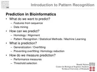
Introduction to Pattern Recognition for Human ICT Review of Linear Algebra. 2014. 9. 12 Hyunki Hong. Contents. Vector and matrix notation Vectors Matrices Vector spaces Linear transformations Eigenvalues and eigenvectors. Vector and matrix notation.

E N D
Introduction to Pattern Recognition for Human ICTReview of Linear Algebra 2014. 9. 12 Hyunki Hong
Contents • Vector and matrix notation • Vectors • Matrices • Vector spaces • Linear transformations • Eigenvalues and eigenvectors
Vector and matrix notation • A 𝑑-dimensional (column) vector 𝑥 and its transpose are written as: • An 𝑛×𝑑 (rectangular) matrix and its transpose are written as • The product of two matrices is cf. The matrix product is associative. If three matrices A, B, and C are respectively m×p, p×q, and q×r matrices, then there are two ways of grouping them without changing their order, and ABC = A(BC) = (AB)C is an m × r matrix.
Vectors also known as • The inner product (a.k.a. dot product or scalar product) of two vectors is defined by: • The magnitude of a vector is • The orthogonal projection of vector 𝑦 onto vector 𝑥 is <𝑦T, 𝑢𝑥>𝑢𝑥. where vector 𝑢𝑥has unit magnitude and the same direction as 𝑥 • The angle between vectors 𝑥 and 𝑦 is • Two vectors 𝑥 and 𝑦 are said to be 1. orthogonal if 𝑥𝑇𝑦 = 0 2. orthonormal if 𝑥𝑇𝑦 = 0 and |𝑥| = |𝑦| = 1 ex)
Vectors • A set of vectors 𝑥1, 𝑥2, …, 𝑥𝑛are said to be linearly dependent if there exists a set of coefficients 𝑎1, 𝑎2, …, 𝑎𝑛(at least one different than zero) such that 𝑎 1 𝑥 1 + 𝑎2 𝑥 2+ … + 𝑎𝑛𝑥𝑛= 0 • Alternatively, a set of vectors 𝑥1, 𝑥2, …, 𝑥𝑛are said to be linearly independent if 𝑎 1 𝑥 1 + 𝑎2 𝑥 2 + … + 𝑎𝑛𝑥𝑛= 0 ⇒ 𝑎𝑘= 0 ∀𝑘
Matrices • The determinant of a square matrix 𝐴𝑑×𝑑is where 𝐴𝑖𝑘is the minor formed by removing the ith row and the kthcolumn of 𝐴 NOTE) The determinant of a square matrix and its transpose is the same: |𝐴|=|𝐴𝑇| • The trace of a square matrix 𝐴𝑑×𝑑is the sum of its diagonal elements. • The rank of a matrix is the number of linearly independent rows (or columns). • A square matrix is said to be non-singular if and only if its rank equals the number of rows (or columns). 1. A non-singular matrix has a non-zero determinant.
Matrices • A square matrix is said to be orthonormal if 𝐴𝐴𝑇 = 𝐴𝑇𝐴 = 𝐼 • For a square matrix 𝐴 1. if 𝑥𝑇𝐴𝑥 > 0 ∀𝑥≠0, then 𝐴 is said to be positive-definite (i.e., the covariance matrix) 2. 𝑥𝑇𝐴𝑥 ≥ 0 ∀𝑥≠0, then 𝐴is said to be positive-semi-definite • The inverse of a square matrix 𝐴 is denoted by 𝐴−1 and is such that 𝐴𝐴−1 = 𝐴 −1 𝐴 = 𝐼 1. The inverse 𝐴−1 of a matrix 𝐴 exists if and only if 𝐴 is non-singular. • The pseudo-inverse matrix 𝐴† is typically used whenever 𝐴−1 does not exist (because 𝐴 is not square or 𝐴 is singular). 1. One-sided inverse (left inverse or right inverse) If the matrix 𝐴 has dimensions and is full rank then use the left inverse if and the right inverse if cf. Formally, given a matrix and a matrix , is a generalized inverse of if it satisfies the condition
Vector spaces • The n-dimensional space in which all the n-dimensional vectors reside is called a vector space. • A set of vectors {𝑢1, 𝑢2, …, 𝑢𝑛} is said to form a basis for a vector space if any arbitrary vector 𝑥can be represented by a linear combination of the {𝑢𝑖} 𝑥 = 𝑎1𝑢 1 + 𝑎2𝑢 2 + ⋯ + 𝑎𝑛𝑢𝑛 1. The coefficients {𝑎1, 𝑎2, …, 𝑎𝑛} are called the components of vector 𝑥 with respect to the basis {𝑢𝑖}. 2. In order to form a basis, it is necessary and sufficient that the {𝑢𝑖} vectors be linearly independent. • A basis {𝑢𝑖} is said to be orthogonal if • A basis {𝑢𝑖} is said to be orthonormal if 1. As an example, the Cartesian coordinate base is an orthonormal base.
Vector spaces • Given n linearly independent vectors {𝑥1, 𝑥2, …, 𝑥𝑛}, we can construct an orthonormal base {𝜙 1, 𝜙 2, …, 𝜙𝑛}for the vector space spanned by {𝑥𝑖} with the Gram-Schmidt orthonormalization procedure. • The distance between two points in a vector space is defined as the magnitude of the vector difference between the points This is also called the Euclidean distance.
Linear transformations • A linear transformation is a mapping from a vector space 𝑋𝑁onto a vector space 𝑌𝑀, and is represented by a matrix. 1. Given vector 𝑥 𝜖 𝑋𝑁, the corresponding vector y on 𝑌𝑀is computed as 2. Notice that the dimensionality of the two spaces does not need to be the same. 3. For pattern recognition we typically have 𝑀<𝑁 (project onto a lower-dimensional space).
Linear transformations • A linear transformation represented by a square matrix 𝐴is said to be orthonormal when 𝐴𝐴𝑇=𝐴𝑇𝐴=𝐼 1. This implies that 𝐴𝑇=𝐴−1 2. An orthonormal x form has the property of preserving the magnitude of the vectors 3. An orthonormal matrix can be thought of as a rotation of the reference frame. ex) 선형변환 추가자료 참조 The rotation takes the vector (1,0) to (cosθ, sinθ) and the vector (0, 1) to (cosθ, -sinθ) . This is just what we need, since in a matrix the first column is just the output when you put in a unit vector along the x-axis; the second column is the output for a unit vector along the y-axis, and so on. So the 2D rotation matrix is.. (cf. 시계방향이면,..)
Eigenvectors and eigenvalues • Given a matrix 𝐴𝑁×𝑁, we say that 𝑣 is an eigenvector* if there exists a scalar 𝜆 (the eigenvalue) such that 𝐴𝑣 = 𝜆𝑣 • Computing the eigenvalues * The "eigen-" in "eigenvector" translates as "characteristic“.
• The matrix formed by the column eigenvectors is called the modal matrix M 1. Matrix Λ is the canonical form of A: a diagonal matrix with eigenvalues on the main diagonal • Properties 1. If Λ is non-singular, all eigenvalues are non-zero. 2. If Λ is real and symmetric, all eigenvalues are real. The eigenvectors associated with distinct eigenvalues are orthogonal. 3. If Λ is positive definite, all eigenvalues are positive
• If we view matrix 𝐴 as a linear transformation, an eigenvector represents an invariant direction in vector space. 1. When transformed by 𝐴, any point lying on the direction defined by 𝑣 will remain on that direction, and its magnitude will be multiplied by 𝜆. 2. For example, the transform that rotates 3-d vectors about the 𝑍 axis has vector [0 0 1] as its only eigenvector and 𝜆 = 1 as its eigenvalue.
• Given the covariance matrix Σ of a Gaussian distribution 1. The eigenvectors of Σ are the principal directions of the distribution. 2. The eigenvalues are the variances of the corresponding principal directions • The linear transformation defined by the eigenvectors of Σ leads to vectors that are uncorrelated regardless of the form of the distribution. 1. If the distribution happens to be Gaussian, then the transformed vectors will be statistically independent.
01_벡터 이론 • 벡터의 표현 • 벡터 : 크기와 방향을 가지는 임의의 물리량 • 패턴 인식에서는 인식 대상이 되는 객체가 특징으로 표현되고, 특징은 차원을 가진 벡터로 표현된다. 이러한 벡터를 특징 벡터(feature vector)라고 한다. • 특징 벡터에 대한 대수학적 계산을 위해서 특징 벡터를 행렬로 표현하여 d차원 공간상의 한 점의 데이터로 특징을 다루게 된다.
01_벡터 이론 • 벡터의 전치 (transpose) • N×1행렬을 1×N행렬로, 혹은 1×N 행렬을 N×1행렬로 행과 열을 바꾼 행렬 • 벡터의 크기 • 원점에서 벡터 공간상의 한 점까지의 거리 • 단위 벡터 • 벡터의 크기가 1인 벡터. • 만약, 벡터 v가 0이 아닌 벡터라면 v방향의 단위벡터 u • 벡터 v방향의 단위 벡터계산: 정규화
01_벡터 이론 • 벡터의 곱셈 내적, 외적 • 스칼라곱 • 임의의 벡터에 임의의 스칼라(실수)를 곱하기 • 내적 (dotproduct) • 차원이 동일한 두 개의 벡터 A,B에 대하여 대응되는 성분 별로 곱하여 합하는 것을두 벡터의 '내적'이라고 함 • 벡터의 내적의 결과는 실수 스칼라 • 두 벡터 사이의 각 θ가 주어질 경우, 내적 스칼라 C = BTA
01_벡터 이론 • 외적 • A,B∈R3 (A,B가 3차원 벡터 공간상에 속한다)인 벡터 A,B가 다음과 같음 • 벡터 외적의 크기는 A와 B를 이웃하는 두 변으로 하는 평행 사변형의 면적과 같음 • 외적의 결과는 A와 B에 동시에 수직이며, 오른손의 엄지와 인지와 중지를 서로 수직이 되게 펴서 인지를 A방향, 중지를 B방향으로 할 때 엄지의 방향을 가르치는 벡터가 됨.
01_벡터 이론 • 단위벡터의 내적 및외적 z k j y i x
01_벡터 이론 • 수직 사영(vectorprojection) • 벡터 x 에 대한 벡터 y의방향성분 • y 벡터를 x 벡터로사영 벡터 x의 방향으로의 방향성분 계산 • 사영 벡터는 내적의 정의를 사용하여 다음과 같이 정의 • ux은 x와 같은 방향의 단위 크기를 가지는 단위 벡터 • 두 벡터 x와 y가 만약, xTy = 0 이면 두 벡터 x와 y는 수직(orthogonal) • xTy = 0 이고 |x |= |y |= 1 이면, 두 벡터 x와 y는 정규 직교(orthonormal) • Ex: 각 좌표축 방향으로의 방향벡터 ◀ 벡터의 내적
01_벡터 이론 • 선형 결합 • 벡터 집합 {x1,x2,…,xm} 과 스칼라 계수 집합 {α1, α2,…, α m} 과의 곱의 합으로 표현된 결과를 벡터 x의 ‘선형 결합(linear combination)’ 혹은 ‘1차 결합’ 이라고 함 • 선형 종속과 선형 독립 • 선형 종속 (linearlydependent) • 임의의벡터 집합을 다른 벡터들의 선형 결합으로 표현할 수 있다면, 이 벡터 집합은 '선형 종속(linearly dependent)'이라고 함 • <{a1, a2, …, am}, {x1,x2,…,xm}> = 0 • 선형 독립 (linearlyindependent) • 만약, 아래식을 만족하는 유일한 해가 모든 i에 대하여 αk = 0, {x1, x2, …, xm} 는 '선형 독립(linearly independent)'이라고 함
01_벡터 이론 • 기저 집합 • N차원의 모든 벡터를 표현할 수 있는 기본벡터의 집합 • 임의의 벡터는 기저 벡터 집합을 통하여 N×1 벡터 공간에 펼쳐진다고 표현 (span) • 만약, {vi}1≤i≤N이 기저 벡터 집합이라면, 임의의 N×1 벡터 x는 다음과 같이 표현함 • 임의의 벡터 x가 {ui} 의 선형 조합으로 표현된다면벡터 집합 {u1, u2, …, un}을N차원 공간의 기저(basis) 라고 함. • 벡터집합 {ui}이기저벡터가 되기 위해서는 서로 선형 독립이어야 함. • 다음 조건을 만족하면 기저 {ui}는 직교 • 다음 조건을 만족하면 기저 {ui}는 정규직교 • 직각좌표계의 단위벡터
01_벡터 이론 • 그램-슈미트 정규 직교화 (Gram-schmidtOrthonormalization) • 서로 선형 독립인 n개의 기저 벡터 {x1, x2, …, xm} 가주어졌을때, 정규직교(orthonormal) 기저 벡터 집합 {p1, p2, …, pn} 을 계산하는 과정 • 기저 직교기저로 변환하는 과정 • {v1, …, vn} 을 벡터공간 V의 기저(basis)라고 하면, 직교벡터 집합 {u1, …, un}은 다음 관계로부터 계산 가능 • V에 대한 정규직교기저(orthonormalbasis)는 각각의 벡터 u1, …, un 을 정규화하면 됨. 정규 직교벡터
01_벡터 이론 • 그램-슈미트 정규 직교화 (Gram-schmidtOrthonormalization) • Example:
01_벡터 이론 • 유클리디안 거리 • 벡터 공간상에서 두 점 간의 거리는 점 사이 벡터 차의 크기로 정의
01_벡터 이론 • 벡터 공간, 유클리드 공간,함수 공간, 널 공간 (null space) • 모든 n차원 벡터들이 존재하는 n차원 공간 • 실제, 벡터 공간은 실수에 의하여 벡터 덧셈과 곱셈에 대한 규칙에 닫혀있는 벡터 집합 • 그러므로 임의의 두 벡터에 대한 덧셈과 곱셈을 통하여 해당 벡터 공간 내에 있는 새로운 벡터를 생성할 수 있음 • 즉, n차원 공간 Rn은 모두 선형독립인 n개의 n차원 벡터에 의해 생성될 수 있음 • 이 때 n차원 공간 Rn을 '유클리드n차원 공간' 혹은 '유클리드 공간'이라고 함 • 벡터의 차원이 무한대일 경우, 벡터 공간은 ‘함수 공간’이 됨 • 행렬 A의 널 공간은 Ax = 0를 만족하는 모든 벡터 x로 이루어져 있는 공간을 뜻한다.
02_행렬 대수 • 전치행렬 (transpose) • 정방행렬 (square matrix) • 행의 수와 열의 수가 동일한 행렬
02_행렬 대수 • 대각 행렬 (diagonal matrix) • 행렬의 대각 성분을 제외하고는 모두 0인 행렬 • 스칼라 행렬 : 대각 성분이 모두 같고, 비대각 성분이 모두 0인 정방행렬 • 항등 행렬 혹은 단위 행렬 (identity matrix) • 대각 성분이 모두 1이고 그밖의 성분이 모두 0인 정방행렬
02_행렬 대수 • 대칭 행렬 (symmetric matrix) • 대각선을 축으로 모든 성분이 대칭되는 행렬 • 영 행렬 • 모든 구성 성분이 0인 행렬 • 직교 행렬 (orthogonal matrix) • 주어진 행렬 A가 정방행렬일 때, 를 만족하는 행렬 • 행렬의각 열(column)이 서로 직교 • 회전 변환과 관계 있는 경우가 많음. 대칭행렬 예: 공분산행렬 Det= 1: rotational transformation Det= -1: reflective transformation, or axis permutation. For an orthogonal matrix, 정방행렬 A의 각 행벡터(또는 열벡터)들이 상호직교인 단위벡터(orthonormal vector)로 이루어짐.
02_행렬 대수 • 행렬의 곱셈 • 행렬의 트레이스(trace)– 정방행렬에서 대각 성분의 합 • 행렬의 고유값 문제에서 고유근을 구할 때 매우 중요한 역할을 함
02_행렬 대수 • 행렬의 계수(rank) • 행렬에서 선형 독립인 열벡터(혹은 행벡터)의 개수 • 다음과 같은 정방행렬 A가 주어질 경우, • 행렬 A 는 세 개의 열벡터 e1, e2, e3 를 사용하여 A = (e1, e2, e3) 로 표현할 수 있음 • 행렬 A 의 계수는 정의에 의해 이들 열벡터 중에서 선형 독립인 벡터의 개수를 말함 • A 행렬은세 벡터가 모두 단위 벡터이고 모두 선형 독립이므로 rank(A) = 3 • 행렬의 계수는 주어진 행렬의 행의 수나 열의 수보다 클 수 없음 • rank(An × n) = n 행렬 A는 비특이(nonsingular)행렬 혹은 정칙행렬 • rank(An × n) < n 행렬 A는 특이(singular)행렬 • 역행렬이 존재하지 않음. (not invertible, rank deficient, degenerate, etc…)
02_행렬 대수 또는행렬값 • 행렬식 (determinant) • 행렬식은 행렬을 어떠한 하나의 실수 값으로 표현한 것을 말함 • d×d정방 행렬 A에 대해행렬식은 |A|혹은 detA 으로 표현하며 다음과 같은 성질을 가짐 • 행렬식은 오직 정방 행렬에서만 정의된다. • 구성 성분이 하나인 행렬의 행렬식은 그 성분 자체이다. • 행렬식의 값은 하나의 상수 즉, 임의의 실수이다. • n차의 행렬식 |An×n| 은 n개의 행과 열의 위치가 서로 다른 성분들의 곱의 합으로 표현된다. • 2x2 행렬의 행렬식 • 3x3 행렬의 행렬식
02_행렬 대수 • 소행렬식 (minor) • 행렬에서i번째 열과 j번째 행을 제거함으로써 얻는 행렬 • 행렬식 계산의 일반화 • 여기서 |Mij| 를 i번째 열과 j번째 행을 제거함으로써 얻어지는 소행렬식이라고 함 • 임의의 행이나 열을 중심으로 전개하여도 결과는 같음 라플라스(Laplace) 전개 • 라플라스 전개 시 부호 • aij의 아래첨자 혹은 소행렬식 |Mij|의 아래첨자의 합이 짝수면 +, 홀수면 -가 됨 • 소행렬식|Mij|에 부호 부분 (-1)i+j까지 곱한 항을 여인수 Aij라고 함
02_행렬 대수 • Ai | j 를 d x d 행렬이라고 할 때 소행렬식으로 A의 행렬식은 순환적으로 구할 수 있음 • i번째 행을 중심으로 전개 • 행렬식의 성질 • 삼각행렬의 행렬식의 값은 대각 성분의 곱 • 전치행렬의 행렬식은 원래 행렬의 행렬식과 같다.
02_행렬 대수 • 역행렬(inversematrix) • 대수 연산에서 임의의 수를 곱하여 1이 될 때, 이를 '역수'라고 함 • 역수를 행렬 대수에 적용했을 때, AX = I 가 되는 X가 존재할 경우에 이 행렬 X를 A의 역행렬이라고 하며 A-1 로 표현한다. • 역행렬의 성질
02_행렬 대수 • 고유값과 고유벡터 (eigenvalues and eigenvectors) • 행렬 A가 n×n의 정방 행렬이고, x ≠ 0인 벡터 x ∈ Rn가 존재할 때 • 다음 관계를 만족하는 스칼라 λ를 행렬 A의 고유값이라고 함 • 벡터 x는 λ에 대응하는 A의 고유 벡터라고 함 • 고유값의 계산 • 동차일차 연립방적식Ax = 0에서 x = 0이 아닌 해를 얻는 유일한 경우는 |A| = 0인 경우 • 따라서 위 식을 만족하려면 |A –λI| = 0일 때 x ≠0 인 해가 존재하게 된다. • 이때 |A –λI| = 0이라는 식을 A의 '특성 방정식'이라고 함 • A를 n×n행렬이라 하고, λ를 A의 고유값이라고 한다. • N개의 고유값과 고유 벡터를 구할 수 있다. • 고유벡터로 정의되는 부분 공간을 A의 고유 공간이라고 한다.
02_행렬 대수 • 고유값과 고유벡터 (eigenvalues and eigenvectors) • 기하학적의미 행렬(선형변환) A의 고유벡터는 선형변환 A에 의해 방향은 보존되고 스케일(scale)만 변화되는 방향 벡터를 나타내고, 고유값은 그 고유벡터의 변화되는 스케일 정도를 나타내는 값. 예) 지구의 자전운동과 같이 3차원 회전변환을 생각했을 때, 이 회전변환에 의해 변하지 않는 고유벡터는 회전축 벡터이고 그 고유값은 1
02_행렬 대수 • 고유값과 고유벡터 (eigenvalues and eigenvectors) • Application example In this shear mapping, the red arrow changes direction but the blue arrow does not. Therefore the blue arrow is an eigenvector, with eigenvalue 1 as its length is unchanged
02_행렬 대수 • 고유값과 고유벡터의 성질 • 대각 행렬의 고유값은 대각 성분 값이다 • 삼각 행렬의 고유값은 이 행렬 대각 성분 값이다 • 벡터 x가 행렬 A의 고유 벡터이면 벡터 x의 스칼라 곱인 kx도 고유 벡터이다 • 전치하여도 고유값은 변하지 않는다. • 행렬 A의 고유값과 전치 행렬 AT 의 고유값은 동일하다 • 역행렬의고유값은 원래 행렬의 고유값의 역수가 된다. • 행렬 A의 모든 고유값의 곱은 A의 행렬식과 같다 • 서로 다른 고유값과 관련된 고유 벡터는 선형 독립이다. • 실수 대칭행렬의 고유 벡터는 서로 직교한다. • 실수 대칭 행렬의 고유값 또한 실수이다. • 만약 A가 양의 정부호 행렬이라면 모든 고유값은 양수이다.
02_행렬 대수 • 고유값과 고유벡터 (eigenvalues and eigenvectors)
02_행렬 대수 • 대각화와 특이벡터, 특이값 • A의 고유값이 λ1, …, λn ,이에 대응하는 1차 독립인 고유벡터가 v1, …, vn 이라고 할 때, C를 다음과 같이 v1, …, vn 을 열벡터로 하는 행렬이라고 하자. • Avn = λnvn이므로, 행렬 곱셈을 열로 표현하면 다음을 얻을 수 있다. • n×n행렬 A가 n개의 1차 독립인 고유벡터를 가진다면, 이 고유벡터들은 A를 대각화하는 행렬 C의 열들로 사용될 수 있다. 그리고 대각행렬은 A의 고유값을 대각원소로 가진다. AC = CΛ → A = CΛC-1 : 행렬 A는 자신의 고유벡터들을 열벡터로 하는 행렬과 고유값을 대각원소로 하는 행렬의 곱으로 대각화 분해 가능 =eigen decomposition 행렬 A의대각화
02_행렬 대수 • 2차 형식 • 3개의 변수 x, y, z의 2차 형식(quadratic form)은 다음과 같은 동차 함수식을 말함 • 2차 함수이기 때문에 2차 형식이라고 한다. F = ax2 + by2 + cz2 + 2fxy + 2gyz + 2hzx • 행렬을 이용하여 표시하면 • 일반화하면 • x=(x1, x2, …, xn), A = (aij)라고 할 때
02_행렬 대수 • SVD : 특이값 재구성 (SingularValue Decomposition) • 어떤 n×m행렬 A는 다음과 같은 형태의 세 가지 행렬의 곱으로 재구성할 수 있다 • U는 특이 벡터를 이루는 열로 구성되며, VT는 특이 벡터를 이루는 행으로 구성된다. • m×m행렬 U의 행은 AAT 의 고유 벡터. • n×n행렬 V의 행은 ATA 의 고유 벡터. • Σ은 n×m인 대각행렬로, 대각성분은 0이 아닌 양수로 구성되며, 이 대각성분을 특이값이라고 한다. • Σ의 특이값들은 AAT와 ATA 의 고유값의 자승근에 해당한다. • 영이 아닌 특이값의 수는 행렬 A의 행렬의 계수(rank)와 같다.
† Singular Value Decomposition A matrix A can be factorized as the following form: U and V are orthogonal, and Σ is diagonal. det = 1: rotational transformation det = -1: reflective transformation, or axis permutation. (orthogonal)
참조: Singular Value Decomposition (SVD) • A rectangular matrix A can be broken down into the product of three matrices: an orthogonal matrix U, a diagonal matrix S, and the transpose of an orthogonal matrix V. Amn = UmmSmnVnnT , where UTU = I, VTV = I ; the coloumns of U are orthonormal eigenvectors of AAT, the columns of V are orthonormal eigenvectors of ATA. S is a diagonal matrix containing the square roots of eigenvalues from U or V in descending order. • Example - To find U, we have to start with AAT.
참조: Singular Value Decomposition (SVD) - To find the eigenvalues & corresponding eigenvectors of AAT. - For λ= 10, For λ= 12, - These eigenvectors become column vectors in a matrix ordered by the size of the corresponding eigenvalue. - Convert this matrix into an orthogonal matrix which we do by applying the Gram-Schmidt orthonormalization process to the column vectors.
참조: Singular Value Decomposition (SVD) 1) Begin by normalizing v1. 2) normalize - The calculation of V: 1) find the eigenvalues of ATA by λ = 0, 10, 12
참조: Singular Value Decomposition (SVD) 2) λ = 12일때, v1 = [1, 2, 1] λ = 10일때, v2 = [2, -1, 0] λ = 0일때, v3 = [1, 2, -5] 3) an orthonormal matrix 4) Amn = UmmSmnVnnT