Download
1 / 13
130 likes | 292 Vues
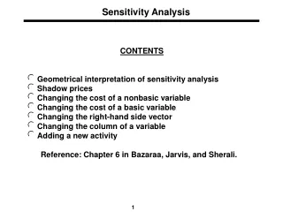
Chapter 8 Sensitivity Analysis. Bottom line: How does the optimal solution change as some of the elements of the model change? For obvious reasons we shall focus on Linear Programming Models. Ingredients of LP Models. Linear objective function A system of linear constraints RHS values

E N D
Chapter 8Sensitivity Analysis • Bottom line: • How does the optimal solution change as some of the elements of the model change? • For obvious reasons we shall focus on Linear Programming Models.
Ingredients of LP Models • Linear objective function • A system of linear constraints • RHS values • Coefficient matrix (LHS) • Signs (=, <=, >=) • How does the optimal solution change as these elements change?
Parametric Changes • Changes in one or more of the coefficients of the objective function (cj)
8.4.3 Changes in the elements of the cost vector, c. • Suppose that the value of ck changes for some k. How will this affect the optimal solution to the LP problem? • We therefore can distinguish between two cases: (1) xk is not in the old basis (2) xk is in the old basis
Case 1: xk is not in the old basis • Thus Recipe: rk >= , if opt=max rk <= , if opt = min
Observations • r’j = 0 for basic variables xj. • (ek)j = 0 for all nonbasic variables xj. • if opt=max all the old reduced costs are non-negative • if opt=min all the old reduced costs are non-positive.
8.4.3 Example Suppose that the reduced costs in the final simplex tableau are as follows: r = (0,0,0,2 3 4) with IB=(2,3,1), namely with x2,x3 and x1 comprising the basis. What would happen if we change the value of c4 ? First we observe that x4 is not in the basis (why?) and that the opt=max
The recipe for this case, namely (8.20) is that the old optimal solution remains optimal as long as r4 ≥ , or in our case, 2 ≥ . • Note that we do not need to know the current (old) value of c4 to reach this conclusion. • Next, suppose that consider changes in c1, recalling that x1 is in the basis.
Preliminary Analysis • We see that in order to analyse this case we have to know the entries in the row of the final tableau which is represented by x1 in the basis (tp.). • What is the value of p? • Since IB=(2,3,1), this is row p=3. • Suppose that this row is as follows: • t3. = (0,0,1,3,-4,0)
We can display this in a "tableau" form as follows: If we add to the old c1, we would have instead correction So we now have to restore the canonical form of the x1 column.
end result .... • To ensure that the current basis remains optimal we have to make sure that all the reduced costs are non-negative (opt=max). Hence, • 2+3 ≥ 0 and 3-4 ≥ 0 • Thus, 3/4 ≥ ≥ -2/3
in words, .... • the old optimal solution will remain optimal if we keep the increase in c1 in the interval [-2/3, 3/4]. If is too small it will be better to enter x4 into the basis, if is too large it will better to put x5 into the basis.