Download
1 / 67
670 likes | 774 Vues
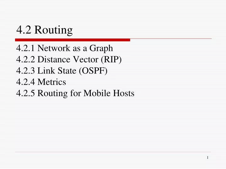
4.2 Routing. 4.2.1 Network as a Graph 4.2.2 Distance Vector (RIP) 4.2.3 Link State (OSPF) 4.2.4 Metrics 4.2.5 Routing for Mobile Hosts. Route a way or course taken in getting from a starting point to a destination send or direct along a specified course Routing

E N D
4.2 Routing 4.2.1 Network as a Graph 4.2.2 Distance Vector (RIP) 4.2.3 Link State (OSPF) 4.2.4 Metrics 4.2.5 Routing for Mobile Hosts
Route • a way or course taken in getting from a starting point to a destination • send or direct along a specified course • Routing • find the path or course of forwarding according to information contained in packet (destination) • Difference between network-layer and link-layer • format of forwarding table • way of updating the table
Link-layer • Forwarding table • mapping from destination physical address (MAC address) to port of forwarding • Update of the table • manually configured
IP (Network) Layer • Forwarding table • mapping from destination network id (NetNum) to next-hop (or interface) of forwarding • Update the table • manually configured (static route) • dynamically learned from routing protocol
Forwarding vs. Routing • Forwarding • taking a packet looking at its destination address consulting a table sending the packet in a direction determined by that table • locally done at a node • Routing • the process by which forwarding tables are built • depends on a distributed algorithm
Forwarding Table vs. Routing Table • Forwarding table • used when a packet is being forwarded and so must contain enough information to accomplish the forwarding function • a row in the forwarding table contains the mapping from a network number to an outgoing interface and some MAC information, such as the Ethernet address of the next hop
Routing table • the table that is built up by the routing algorithms as a precursor to building the forwarding table • it contains mappings from network numbers to next-hops (IP addresses)
Example, in the following tables • the routing table tells us that network number 10 is to be reached by a next hop router with the IP address 171.69.245.10 • the forwarding table contains the information about exactly how to forward a packet to that next hop • send it out interface number 0 with a MAC address of 8:0:2b:e4:b:l:2 (the last piece of information is provided by the Address Resolution Protocol)
(b) (a) Example rows from (a) routing and (b) forwarding tables
Basic problem of routing • find the lowest-cost path between any two nodes, where the cost of a path equals the sum of the costs of all the edges that make up the path
Solution • routing is achieved in most practical networks by running routing protocols among the nodes • these protocols provide a distributed, dynamic way to solve the problem of finding the lowest-cost path in the presence of • node or link failure • addition of new node or new link • changes of link cost • it is difficult to make centralized solutions scalable, so all the widely used routing protocols use distributed algorithms
4.2.2 Distance Vector (RIP) • Distance-Vector Algorithm (Bellman-Ford Algorithm) • each node constructs a one-dimensional array (a vector) containing the "distances" (costs) to all other nodes and distributes that vector to its immediate neighbors • response when receiving an announcement from a neighbor • for every entry in the announcement, store it if • the announced distance is shorter than what in the table • a better route is found • otherwise discard it
assumption • initially, each node knows the cost of the link to each of its directly connected neighbors • broken links are assigned an infinite cost, ∞
Local data structure • routing table • destination • cost to the destination • corresponding next-hop
Distance Vector Algorithm • In this example • the cost of each link is set to 1 • a least-cost path is simply the one with the fewest hops
B A C E D F G Initial State
A’s routing table B A C E D F G Distance Vector sent by A
B A C E D F G After One Step
B A C E D F G After Two Steps convergence: no more changes when getting further announcement
Two different circumstances for a node to send a routing update to its neighbors • periodic update • each node automatically sends an update message every so often, even if nothing has changed • triggered update • happens whenever a node receives an update from one of its neighbors that causes it to change one of the routes in its routing table • i.e., whenever a node's routing table changes, it sends an update to its neighbors, which may lead to a change in their tables, causing them to send an update to their neighbors
Link Failures • Example 1 (stable) • F detects that link to G has failed • F sets distance to G to infinity and sends update to A [F:(G, ∞, G)] • A sets distance to G to infinity since it uses F to reach G [A:(G, ∞, F)] ------------------------------------------------------------------------- • A receives periodic update from C with 2-hop path to G • A sets distance to G to 3 and sends update to F[A:(G, 3, C)] • F decides it can reach G in 4 hops via A[F:(G, 4, A)] Pattern:(Dest, Cost, NextHop)
∞ • Example 2 (count to infinity) • link from A to E fails • A advertises distance of infinity to E [A:(E, ∞, E)] • B and C advertise a distance of 2 to E [B:(E, 2, A)] ,[C:(E, 2, A)] • B hears that E can be reached in 2 hops from C • B decides it can reach E in 3 hops; advertises this to A [B:(E, 3, C)] • A decides it can reach E in 4 hops; advertises this to C[A:(E, 4, B)] • C decides that it can reach E in 5 hops… [C:(E, 5, A)]
Loop-breaking heuristics (partial solutions) • set infinity to 16 • split horizon • split horizon with poison reverse
Solution-1 (set infinity to 16) • use some relatively small number as an approximation of infinity, which at least bounds the amount of time that it takes to count to infinity • example, set the maximum number of hops to get across a certain network is never going to be more than 16 (set 16 to be infinity value) • drawback • problem occurs if our network grew to a point where some nodes were separated by more than 16 hops
Solution-2 (split horizon) • when a node sends a routing update to its neighbors, it does not send those routes it learned from each neighbor back to that neighbor • example, if B has the route (E, 2, A) in its table, then it knows it must have learned this route from A, and so whenever B sends a routing update to A, it does not include the route (E, 2, A) in that update
Solution-3 (split horizon with poison reverse) • (B actually sends that route back to A, but it puts negative information in the route to ensure that A will not eventually use B to get to E) • Let B be a neighbor of A • if in the routing table of B, the next hop entry for destination Z is A, B informs A that its distance to Z is infinite[B:(Z, cost, A) → A:(Z, ∞, B)]
Solution 2 & 3 only work for routing loops that involve two nodes • example, for larger routing loops • if B and C had waited for a while after hearing of the link failure from A before advertising routes to E • they would have found that neither of them really had a route to E
Routing Information Protocol (RIP) • One of the most widely used routing protocols in IP networks • A DV (Distance Vector) routing protocol • Rather than advertising the cost of reaching other routers, the routers advertise the cost of reaching networks • example, in the following figure, router C would advertise to router A the fact that it can reach • networks 2 and 3 at cost 0 [C:(Net2, 0, Net2),C:(Net3, 0, Net3)] • networks 5 and 6 at cost 1[C:(Net5, 1, Net3),C:(Net6, 1, Net3)] • network 4 at cost 2[C:(Net4, 2, Net3)]
RIP packet format • the majority of the packets is taken up with (network-address, distance) pairs • example • if router A learns from router B that network X can be reached at a lower cost via B than via the existing next hop in the routing table • A updates the cost and next hop information for the network number accordingly
RIP • a fairly straightforward implementation of distance-vector routing • routers running RIP send their advertisements every 30 seconds • a router also sends an update message whenever an update from another router causes it to change its routing table
metrics or costs for routing • all link costs being equal to 1 • always tries to find the minimum hop route • valid distances are 1 through 15, with 16 representing infinity (this limits RIP to running on fairly small networks-those with no paths longer than 15 hops)
4.2.3 Link State (OSPF) • Distance-Vector approach • “tell neighbors where I can go, and how far” • Link-State approach • “tell all which neighbors I have”
Link-state routing • the second major class of intradomain routing protocol • assumptions • each node is assumed to be capable of finding out the state of the link to its neighbors (up or down) and the cost of each link • Intradomain • An internetwork in which all the routers are under the same administrative control (e.g., a single university campus, or the network of a single Internet service provider)
basic idea • every node knows how to reach its directlyconnected neighbors, and if we make sure that the totality of this knowledge is disseminated to every node, then every node will have enough knowledge of the network to build a completemap of the network • link-state routing protocols rely on two mechanisms • reliable dissemination of link-state information • calculation of routes from the sum of all the accumulated link-state knowledge
Link-State Message Data Structure • LSP (Link-State Packet) • an update packet created by each node • information for route calculation • the ID of the node that created the LSP • a list of directly connected neighbors of the node, with the cost of the link to each one
information for reliability • a sequence number • ensure having the most recent copy • reset to zero when routing process restarted • a time to live (TTL) for this packet • Too old packets are discarded
Reliable Flooding • Send local LSP out on all of its directly connected links • Each node receiving the LSP forwards it out on all of its links • stores each node’s recent LSP • forwards LSP to neighbors except the sender itself
The following figure shows an LSP being flooded in a small network • each node becomes shaded as it stores the new LSP (a) the LSP arrives at node X, which sends it to neighbors A and C (b) A and C do not send it back to X, but send it on to B (c) B receives two identical copies of the LSP, it will accept whichever arrived first and ignore the second as a duplicate (d) B passes the LSP onto D, who has no neighbors to flood it to, and the process is complete
New LSP Generation • Two circumstances to generate new LSP • expiry of a periodic timer • change in topology • directly connected links go down • detected by link-layer protocols • immediate neighbors go down • detected by periodic “hello” message
Calculation of Route • Dijkstra’s Shortest Path Algorithm • Notations • N: vertex set of the graph • l: l(i, j) is the (non-negative) cost of the edge (i, j) • s: current vertex • M: set of ever calculated vertices • C(n): cost of path from s to n
Calculate a minimum-cost tree from s M = {s} for each n in N-{s} C(n) = l(s,n) while (N != M) M = M union {w} such that C(w) is the minimum for all w in (N-M) for each n in (N-M) C(n) = MIN(C(n),C(w)+l(w,n))
In practice, each switch computes its routing table directly from the LSPs it has collected using a forward search approach for Dijkstris algorithm • each switch maintains two lists, known as Tentative and Confirmed. • each of these lists contains a set of entries of the form (Destination, Cost, NextHop)
Forward Search Approach for Dijkstra Algorithm 1. Initialize the Confirmed list with an entry for myself; this entry has a cost of 0. 2. For the node just added to the Confirmed list in the previous step, call it node Next, select its LSP. 3. For each neighbor (Neighbor) of Next, calculate the cost (Cost) to reach this Neighbor as the sum of the cost from myself to Next and from Next to Neighbor. • (a) If Neighbor is currently not on either the Confirmed or the Tentative list, then add (Neighbor, Cost, NextHop) to the Tentative list, where NextHop is the direction I go to reach Next. • (b) If Neighbor is currently on the Tentative list, and the Cost is less than the currently listed cost for Neighbor, then replace the current entry with (Neighbor, Cost, NextHop), where NextHop is the direction I go to reach Next. 4. If the Tentative list is empty, stop. Otherwise, pick the entry from the Tentative list with the lowest cost, move it to the Confirmed list, and return to step 2.
Example Link-state routing: an example network
(B, 11, B) → (C, 2, C) (B, 5, C) → (A, 12, C) (A, 10, C)
Open Shortest Path First Protocol (OSPF) • OSPF • one of the most widely used link-state routing protocols • Open: refers to the fact that it is an open, nonproprietary standard, created under the auspices of the IETF • SPF: comes from an alternative name for link-state routing