Download
1 / 44
440 likes | 450 Vues
CprE / ComS 583 Reconfigurable Computing. Prof. Joseph Zambreno Department of Electrical and Computer Engineering Iowa State University Lecture #23 – Function Unit Architectures. Quick Points. Next week Thursday, project status updates 10 minute presentations per group + questions

E N D
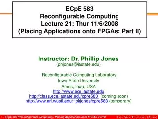
CprE / ComS 583Reconfigurable Computing Prof. Joseph Zambreno Department of Electrical and Computer Engineering Iowa State University Lecture #23 – Function Unit Architectures
Quick Points • Next week Thursday, project status updates • 10 minute presentations per group + questions • Upload to WebCT by the previous evening • Expected that you’ve made some progress! CprE 583 – Reconfigurable Computing
Allowable Schedules Active LUTs (NA) = 3 CprE 583 – Reconfigurable Computing
Sequentialization • Adding time slots • More sequential (more latency) • Adds slack • Allows better balance L=4 NA=2 (4 or 3 contexts) CprE 583 – Reconfigurable Computing
Multicontext Scheduling • “Retiming” for multicontext • goal: minimize peak resource requirements • NP-complete • List schedule, anneal • How do we accommodate intermediate data? • Effects? CprE 583 – Reconfigurable Computing
Signal Retiming • Non-pipelined • hold value on LUT Output (wire) • from production through consumption • Wastes wire and switches by occupying • For entire critical path delay L • Not just for 1/L’th of cycle takes to cross wire segment • How will it show up in multicontext? CprE 583 – Reconfigurable Computing
Signal Retiming • Multicontext equivalent • Need LUT to hold value for each intermediate context CprE 583 – Reconfigurable Computing
Full ASCII Hex Circuit • Logically three levels of dependence • Single Context: 21 LUTs @ 880Kl2=18.5Ml2 CprE 583 – Reconfigurable Computing
Multicontext Version • Three contexts: 12 LUTs @ 1040Kl2=12.5Ml2 • Pipelining needed for dependent paths CprE 583 – Reconfigurable Computing
ASCIIHex Example • All retiming on wires (active outputs) • Saturation based on inputs to largest stage • With enough contexts only one LUT needed • Increased LUT area due to additional stored configuration information • Eventually additional interconnect savings taken up by LUT configuration overhead IdealPerfect scheduling spread + no retime overhead CprE 583 – Reconfigurable Computing
ASCIIHex Example (cont.) @ depth=4, c=6: 5.5Ml2 (compare 18.5Ml2 ) CprE 583 – Reconfigurable Computing
General Throughput Mapping • If only want to achieve limited throughput • Target produce new result every t cycles • Spatially pipeline every t stages • cycle = t • Retime to minimize register requirements • Multicontext evaluation w/in a spatial stage • Retime (list schedule) to minimize resource usage • Map for depth (i) and contexts (c) CprE 583 – Reconfigurable Computing
Benchmark Set • 23 MCNC circuits • Area mapped with SIS and Chortle CprE 583 – Reconfigurable Computing
Area v. Throughput CprE 583 – Reconfigurable Computing
Area v. Throughput (cont.) CprE 583 – Reconfigurable Computing
Reconfiguration for Fault Tolerance • Embedded systems require high reliability in the presence of transient or permanent faults • FPGAs contain substantial redundancy • Possible to dynamically “configure around” problem areas • Numerous on-line and off-line solutions CprE 583 – Reconfigurable Computing
Column Based Reconfiguration • Huang and McCluskey • Assume that each FPGA column is equivalent in terms of logic and routing • Preserve empty columns for future use • Somewhat wasteful • Precompile and compress differences in bitstreams CprE 583 – Reconfigurable Computing
Column Based Reconfiguration • Create multiple copies of the same design with different unused columns • Only requires different inter-block connections • Can lead to unreasonable configuration count CprE 583 – Reconfigurable Computing
Column Based Reconfiguration • Determining differences and compressing the results leads to “reasonable” overhead • Scalability and fault diagnosis are issues CprE 583 – Reconfigurable Computing
Summary • In many cases cannot profitably reuse logic at device cycle rate • Cycles, no data parallelism • Low throughput, unstructured • Dissimilar data dependent computations • These cases benefit from having more than one instructions/operations per active element • Economical retiming becomes important here to achieve active LUT reduction • For c=[4,8], I=[4,6] automatically mapped designs are 1/2 to 1/3 single context size CprE 583 – Reconfigurable Computing
Outline • Continuation • Function Unit Architectures • Motivation • Various architectures • Device trends CprE 583 – Reconfigurable Computing
Coarse-grained Architectures • DP-FPGA • LUT-based • LUTs share configuration bits • Rapid • Specialized ALUs, mutlipliers • 1D pipeline • Matrix • 2-D array of ALUs • Chess • Augmented, pipelined matrix • Raw • Full RISC core as basic block • Static scheduling used for communication CprE 583 – Reconfigurable Computing
DP-FPGA • Break FPGA into datapath and control sections • Save storage for LUTs and connection transistors • Key issue is grain size • Cherepacha/Lewis – U. Toronto CprE 583 – Reconfigurable Computing
0 0 0 1 1 1 1 0 A1 A0 B1 B0 C1 C0 Y0 MC = LUT SRAM bits CE = connection block pass transistors Y1 Set MC = 2-3CE Configuration Sharing CprE 583 – Reconfigurable Computing
Two-dimensional Layout • Control network supports distributed signals • Data routed as four-bit values CprE 583 – Reconfigurable Computing
DP-FPGA Technology Mapping • Ideal case would be if all datapath divisible by 4, no “irregularities” • Area improvement includes logic values only • Shift logic included CprE 583 – Reconfigurable Computing
RaPiD • Reconfigurable Pipeline Datapath • Ebeling –University of Washington • Uses hard-coded functional units (ALU, Memory, multiply) • Good for signal processing • Linear array of processing elements Cell Cell Cell CprE 583 – Reconfigurable Computing
RaPiD Datapath • Segmented linear architecture • All RAMs and ALUs are pipelined • Bus connectors also contain registers CprE 583 – Reconfigurable Computing
RaPiD Control Path • In addition to static control, control pipeline allows dynamic control • LUTs provide simple programmability • Cells can be chained together to form continuous pipe CprE 583 – Reconfigurable Computing
FIR Filter Example • Measure system response to input impulse • Coefficients used to scale input • Running sum determined total CprE 583 – Reconfigurable Computing
FIR Filter Example (cont.) • Chain multiple taps together (one multiplier per tap) CprE 583 – Reconfigurable Computing
MATRIX • Dehon and Mirsky -> MIT • 2-dimensional array of ALUs • Each Basic Functional Unit contains “processor” (ALU + SRAM) • Ideal for systolic and VLIW computation • 8-bit computation • Forerunner of SiliconSpice product CprE 583 – Reconfigurable Computing
Basic Functional Unit • Two inputs from adjacent blocks • Local memory for instructions, data CprE 583 – Reconfigurable Computing
MATRIX Interconnect • Near-neighbor and quad connectivity • Pipelined interconnect at ALU inputs • Data transferred in 8-bit groups • Interconnect not pipelined CprE 583 – Reconfigurable Computing
Functional Unit Inputs • Each ALU inputs come from several sources • Note that source is locally configurable based on data values CprE 583 – Reconfigurable Computing
FIR Filter Example • For k-weight filter 4K cells needed • One result every 2 cycles • K/2 8x8 multiplies per cycle K=8 CprE 583 – Reconfigurable Computing
Chess • HP Labs – Bristol, England • 2-D array – similar to Matrix • Contains more “FPGA-like” routing resources • No reported software or application results • Doesn’t support incremental compilation CprE 583 – Reconfigurable Computing
Chess Interconnect • More like an FPGA • Takes advantage of near-neighbor connectivity CprE 583 – Reconfigurable Computing
Chess Basic Block • Switchbox memory can be used as storage • ALU core for computation CprE 583 – Reconfigurable Computing
Reconfigurable Architecture Workstation • MIT Computer Architecture Group • Full RISC processor located as processing element • Routing decoupled into switch mode • Parallelizing compiler used to distribute work load • Large amount of memory per tile CprE 583 – Reconfigurable Computing
RAW Tile • Full functionality in each tile • Static router located for near-neighbor communication CprE 583 – Reconfigurable Computing
RAW Datapath CprE 583 – Reconfigurable Computing
Raw Compiler • Parallelizes compilation across multiple tiles • Orchestrates communication between tiles • Some dynamic (data dependent) routing possible CprE 583 – Reconfigurable Computing
Summary • Architectures moving in the direction of coarse-grained blocks • Latest trend is functional pipeline • Communication determined at compile time • Software support still a major issue CprE 583 – Reconfigurable Computing