Download
1 / 58
590 likes | 766 Vues
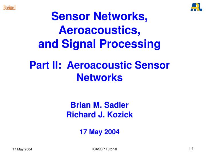
Sensor Networks, Aeroacoustics, and Signal Processing Part II: Aeroacoustic Sensor Networks Brian M. Sadler Richard J. Kozick 17 May 2004. Central Node?. Heterogeneous Network of Acoustic Sensors. One mic. Sensor array. Source. 10’s to 100’s of m range. Issues:

E N D
Sensor Networks, Aeroacoustics,and Signal ProcessingPart II: Aeroacoustic Sensor NetworksBrian M. SadlerRichard J. Kozick17 May 2004 ICASSP Tutorial
Central Node? Heterogeneous Network of Acoustic Sensors One mic. Sensorarray Source 10’s to 100’s of mrange • Issues: • Centralized versus distributed processing • Minimize comms., energy • Triangulation, TDOA? • Effects of acoustic prop. • (Node localization, sensor layout & density, Classification, tracking) ICASSP Tutorial
DSP Acoustic Source & Propagation Signalat sensor (mic.) Source Turbulence scatters wavefronts • Source: • Loud • Spectral lines • One sensor: • Detection • Doppler estimation • Harmonic signature ICASSP Tutorial
DSP More Sophisticated Node:Sensor Array 1 m apertureor (much) less • Issues: • Array size/baseline • Coherence decreases with larger spacing • AOA estimation accuracy with turbulent scattering • What can we do with a hockey-puck sensor? • Small, covert, easily deployable • Performance? Wavelength ~ 1 to 10 m ICASSP Tutorial
Why Acoustics? • Advantages: • Mature sensor technology (microphones) • Low data bandwidth: ~[30, 250] Hz Sophisticated, real-time signal proc. • Loud sources, difficult to hide: vehicles, aircraft, ballistics • Challenges: • Ultra-wideband regime: 157% fractional BW • λ in [1.3, 11] m Small array baselines • Propagation: turbulence, weather, (multipath) • Minimize network communications • We bound the space of useful system design and performance [Kozick2004a] • with respect to SNR, range, frequency, bandwidth, observation time, propagation conditions (weather), sensor layout, source motion/track • evaluate performance of algorithms (simulated & measured data) Distinct fromRF arrays ICASSP Tutorial
Brief History of Acoustics in Military [Namorato2000] • Trumpeting down walls of Jericho • Chinese, Roman (B.C.) • Civil War: Generals used guns to signal attacks • World War 1: • Science of acoustics developed • Air & underwater acoustic systems • World War 2: Mine actuating, submarine detection • Many developments … • Army Research Laboratory, 1991-present [Srour1995] • Hardware and software for detection, localization, tracking, and classification • Extensive field testing in various environments with many vehicle types ICASSP Tutorial
Remainder of Tutorial • A little more background: • Source characteristics • Sound propagation through turbulent atmosphere • Detection of sources (Saturation, W) • Array processing • Coherence loss from turbulence (Coherence, g) • Array size: 2 sensors source AOA • Array of arrays source localizationDistributed processing? Data to transmit?Triangulation/TDOA Minimize comms. Experimentallyvalidatedmodels ICASSP Tutorial
Source Characteristics • Ground vehicles (tanks, trucks), aircraft (rotary, jet), commercial vehicles, elephant herds LOUD • Main contributors to source sound: • Rotating machinery: Engines, aircraft blades • Tires and “tread slap” (spectral lines) • Vibrating surfaces • Internal combustion engines: Sum-of-harmonics due to cylinder firing • Turbine engines: Broadband “whine” • Key features: Spectral lines and high SNR Distinct fromunderwater ICASSP Tutorial
High SNR TIME (sec) +/- 350 m from Closest Point of Approach (CPA) ICASSP Tutorial
Frequency Harmonic lines Doppler shift: 0.5 Hz @ 14.5 Hz 3 Hz @ 87 Hz Time +/- 85 m from CPA CPA = 5 m 15 km/hr ICASSP Tutorial
Overview of Propagation Issues • “Long” propagation time: 1 s per 330 m • Additive noise: Thermal, Gaussian(also wind and directional interference) • Scattering from random inhomogeneities (turbulence) temporal & spatial correl. • Random fluctuations in amplitude: W • Spatial coherence loss (>1 sensor): g • Transmission loss: Attenuation by spherical spreading and other factors ICASSP Tutorial
Numerical Solution[Wilson2002] Transmission Loss • Energy is diminished from Sref (at 1 m from source) to S at sensor: • Spherical spreading • Refraction (wind, temp. gradients) • Ground interactions • Molecular absorption • We model S as a deterministic parameter: Average signal energy Low Pass Filter [Embleton1996] +/- 125 m from CPA ICASSP Tutorial
Measured Aeroacoustic Data ICASSP Tutorial
Measured SNR vs. Range & Frequency dB Time Aspect dependence SNR ~ 50 dB at CPA Fluctuations due to turbulence ICASSP Tutorial
Outline Sinusoidal signal emitted by moving source: • Detection of sources • Saturation, W • Detection performance • Array processing • Coherence loss from turbulence, g • Array size: 2 sensors Source AOA • Array of arrays: Source localizationTriangulation/TDOA, minimize comms. • Propagation delay, t • Additive noise • Transmission loss • Turbulent scattering Signal at the sensor: ICASSP Tutorial
Sensor Signal: No Scattering • Sensor signal with transmission loss,propagation delay, and AWG noise: • Complex envelope at frequency fo • Spectrum at fo shifted to 0 Hz • FFT amplitude at fo ICASSP Tutorial
Sensor Signal: With Scattering • A fraction, W, of the signal energy is scattered from a pure sinusoid into a zero-mean, narrowband, Gaussian random process, : • Saturation parameter, W in [0, 1] • Varies w/ source range, frequency, and meteorological conditions (sunny, windy) • Based on physical modeling of sound propagation through random, inhomogeneous medium • Easier to see scattering effect with a picture: [Norris2001, Wilson2002a] ICASSP Tutorial
Weak Scattering: W ~ 0 Strong Scattering: W ~ 1 (1- W)S Power Spectral Density (PSD) WS Area= WS AWGN, 2No (1- W)S 0 0 Freq. -B/2 B/2 -B/2 B/2 Bv Bv • Study detection of source, w/ respect to • Saturation, W (analogous to Rayleigh/Rician fading in comms.) • Processing bandwidth, B, and observation time, T • SNR = S / (2 No B) • Scattering bandwidth, Bv < 1 Hz (correlation time ~ 1/Bv > 1 sec) • Number of independent samples ~ (T Bv) often small • Scattering (W > 0) causes signal energy fluctuations ICASSP Tutorial
Probability Distributions • Complex amplitude has complex Gaussian PDF with non-zero mean: • Energy has non-central c-squared PDF with 2 d.o.f. • has Rice PDF (Experimental validation in [Daigle1983, Bass1991, Norris2001]) ICASSP Tutorial
Saturation vs. Frequency & Range • Saturation depends on [Ostashev2000]: • Weather conditions (sunny/cloudy), but varies little with wind speed • Source frequency w and range do Theoretical forms Constants from numerical evaluation of particular conditions ICASSP Tutorial
Turbulence effects are small only for very short range and low frequency Saturation variesover entire range[0, 1] for typicalrange & freq.values Fully scattered ICASSP Tutorial
Detection Performance PD = probability of detectionPFA = probability of false alarm Fullscattering Noscattering Scattering beginsto limit performance ICASSP Tutorial
Detection Performance with Range Lower frequenciesdetected at larger ranges SNR = 50 dB at 10 m rangeSNR ~ 1/(range)2 1 km 200 Hz • Saturation increases with • Range • Frequency • Temperature (sunny) 40 Hz ICASSP Tutorial
Detection Extensions • Sensor networks: Detection queuing (wake-up) of more sophisticated sensors • Multiple snapshots & frequencies • Source motion & nonstationarities • Coherence time of scattering • Multiple sensors with different SNR and W • Distributed detection, what to communicate? • Required sensor density for reliable detection • Source localization based on energy level at the sensors [Pham2003] Physical models for cross-freq coherenceand coherence timeare in preliminary stage[Norris2001, Havelock1998] ICASSP Tutorial
Outline • Detection of sources • Saturation, W • Detection performance • Array processing • Coherence loss from turbulence, g • Array size: 2 sensors Source AOA • Array of arrays: Source localizationTriangulation/TDOA, minimize comms. • Coherence, g, depends on • Sensor separation, r • Source frequency, w • Source range, do • Weather conditions: sunny/cloudy, wind speed ICASSP Tutorial
q = AOA • = sensor spacing < l/2 Signal Model forTwo Sensors Turbulence effects Perfect plane wave:W = 0 or 1g = 1 ICASSP Tutorial
q do = range • = sensor spacing Model for Coherence, g • Assume AOA q = 0, freq. in [30, 500] Hz • Recall saturation model: • Coherence model [Ostashev2000]: g 0 with freq., sensorspacing, and range Temperaturefluctuations Velocityfluctuations (wind) ICASSP Tutorial
Velocityfluctuations (wind) Temperaturefluctuations Depends on wind leveland sunny/cloudy (From [Kozick2004a], based on[Ostashev2000, Wilson2000]) ICASSP Tutorial
Assumptions for Model Validity [Kozick2004a] • Line of sight propagation (no multipath) appropriate for flat, open terrain • AWGN is independent from sensor to sensor ignores wind noise, directional interference • Scattered process is complex, circular, Gaussian [Daigle1983, Bass1991, Norris2001] • Wavefronts arrive at array aperture with near-normal incidence • Sensor spacing, r, resides in the inertial subrange of the turbulence: smallest turbulent eddies << r << largest turbulent eddies = Leff ICASSP Tutorial
Coherence, g, versus frequencyand range forsensor spacingr = 12 inches • > 0.99 for range < 100 m.Is this “good”? Curves shiftup w/ less wind,down w/ more wind ICASSP Tutorial
SenTech HE01 acoustic sensor [Prado2002] Outline • Freq. in [30, 250] Hz l in [1.3, 11] m • Angle of arrival (AOA) accuracy w.r.t. • Array aperture size • Turbulence (W, g) • Small aperture: • Easier to deploy • More covert • Better coherence • How small can we go? • Detection of sources • Saturation, W • Detection performance • Array processing • Coherence loss from turbulence, g • Array size: 2 sensors Source AOA • Array of arrays: Source localizationTriangulation/TDOA, minimize comms. ICASSP Tutorial
Impact on AOA Estimation • How does the turbulence (W, g) affect AOA estimation accuracy? [Sadler2004] • Cramer-Rao lower bound (CRB), simulated RMSE • Achievable accuracy with small arrays? Larger sensorspacing, r: DESIRABLE BAD! ICASSP Tutorial
Special Cases of CRB • No scattering (ideal plane wave model): • High SNR, with scattering: SNR-limitedperformance Coherence-limitedperformance If SNR = 30 dB, then g < 0.9989995 limits performance! ICASSP Tutorial
Phase CRB with Scattering ( W, g) Coherence loss g < 1 is significantwhen saturationW > 0.1 Idealplanewave ICASSP Tutorial
CRB on AOA Estimation SNR = 30 dB for all ranges Sensor spacing r = 12 in. Coherence-limited at larger ranges Increasingrange (fixed SNR) Aperture-limitedat low frequency Ideal plane wave modelis accurate for very shortranges ~ 10 m ICASSP Tutorial
Cloudy and Less Wind SNR = 30 dB for all ranges Sensor spacing r = 12 in. Atmospheric conditionshave a large impact onAOA CRBs Aperture-limitedat low frequency Plane wave model isaccurate to 100 m range ICASSP Tutorial
Coherence vs. Sensor Spacing Lightwind Strongwind g = 0 for r ~ 1,000 in = 25 m ICASSP Tutorial
CRB on AOA vs. Sensor Spacing r = 5 inches ICASSP Tutorial
Coherence vs. Sensor Spacing ICASSP Tutorial
CRB on AOA vs. Sensor Spacing Ideal planewave modelis optimistic (poor weather) Coherence lossesdegrade AOA perf.for r > 8 feet (First noted in[Wilson1998], [Wilson1999]) l/2 Plane waveis OK for good weather ICASSP Tutorial
CRB Achievability Phase difference estimator: Scenario:Small Sensor Spacing: r = 3 in., SNR = 40 dB, Range = 50 m AOA estimators break away from CRB approx.when W > 0.1 Saturation W issignificant for most offrequency range Turbulence prevents performance gain from larger aperture Coherence is high: g > 0.999 Aperture-limited ICASSP Tutorial
AOA Estimation for Harmonic Source Equal-strength harmonicsat 50, 100, 150 Hz SNR = 40 dB at 20 mrange, SNR ~ 1/(range)2 (simple TL) Sensor spacingr = 3 in. and 6 in. Mostly sunny,moderate wind One snapshot r = 3 in. RMSE r = 6 in. CRB Achievable AOA accuracy ~ 10’s of degrees for this case ICASSP Tutorial
Turbulence Conditions for Three-Harmonic Example Strongscattering Coherence is ~ 1,but still limits performance. ICASSP Tutorial
Summary of AOA Estimation • CRB analysis of AOA estimation • Tradeoff: larger aperture vs. coherence loss • Ideal plane wave model is overly optimistic for longer source ranges • Performance varies significantly with weather cond. • Important to consider turbulence effects • AOA algorithms do not achieve the CRB in turbulence (W > 0.1) with one snapshot • Similar results obtained for circular arrays with > 2 sensors [Sadler2004] ICASSP Tutorial
Outline • Issues: • Comm. bandwidth • Distributed processing • Exploit long baselines? • Time sync. among arrays • Model assumptions: • Individual arrays: • Perfect coherence • Far-field • Between arrays: • Partial coherence • Different power spectra • Near-field • Detection of sources • Saturation, W • Detection performance • Array processing • Coherence loss from turbulence, g • Array size: 2 sensors Source AOA • Array of arrays: Source localizationTriangulation/TDOA, minimize comms. ICASSP Tutorial
Source Source Fusion Node Fusion Node Fusion Node Three Localization Schemes AOA &TDOA AOA AOA &TDOA AOA Transmit raw data from one sensorto other nodes Source AOA AOA TransmitAOAs Transmitraw data from all sensors TransmitAOAs & TDOAs Noncoherenttriangulationof AOAs Optimum,coherentprocessing Triangulationof AOAs andTDOAs • 2) Fully centralized • Comms.: High • Centralized processing • Fine time sync. req’d • Near-field w.r.t. arrays • 3) AOAs & TDOAs: • Comms.: Medium • Distributed processing • Fine time sync. req’d • Alt.: Each array xmits raw data from 1 sensor • 1) Triangulate AOAs: • Comms.: Low • Distributed processing • Coarse time sync. ICASSP Tutorial
Localization Cramer-Rao Bounds [Kozick2004b] • Triangulation of AOAs Minimal comms. • Fully centralized Maximum comms. • #1 + time delay estimation (TDE) Raw data from 1 sensor • Schemes 2 & 3 have same CRB! • Results are coherence sensitive: coherence improves CRB over AOA triangulation • Are the CRBs achievable? AOAtriangulation Parameters: 3 arrays, 7 elements, 8 ft. diam.Narrowband (49.5 to 50.5 Hz)SNR = 16 dB at each sensor0.5 sec. observation time ICASSP Tutorial
TB product Fract BW SNR Ziv-Zakai Bound on TDE • Threshold coherence to attain CRB: • Function(SNR, % BW, TB product, coherence) • Extends [WeissWeinstein83] to TDE with partially-coherent signals ICASSP Tutorial
Threshold Coherence Simulation Breakaway from CRB is accurately predictedby threshold coherence value ICASSP Tutorial
Threshold Coherence Doubling fractional BW time-BW product reduced by factor of ~ 10 f0 = 50 Hz, Df = 5 Hz T>100 s Narrowband sourcerequires perfect coherence ICASSP Tutorial