Download

1 / 51
970 likes | 2.22k Vues
A PRIORI OR PLANNED CONTRASTS. MULTIPLE COMPARISON TESTS. ANOVA. ANOVA is used to compare means. However, if a difference is detected, and more than two means are being compared, ANOVA cannot tell you where the difference lies.

E N D
A PRIORI OR PLANNED CONTRASTS MULTIPLE COMPARISON TESTS
ANOVA • ANOVA is used to compare means. • However, if a difference is detected, and more than two means are being compared, ANOVA cannot tell you where the difference lies. • In order to figure out which means differ, you can do a series of tests: • Planned or unplanned comparisons of means.
PLANNED or A PRIORI CONTRASTS • A comparison between means identified as being of utmost interest during the design of a study, prior to data collection. • You can only do one or a very small number of planned comparisons, otherwise you risk inflating the Type 1 error rate. • You do not need to perform an ANOVA first.
UNPLANNED or A POSTERIORI CONTRASTS • A form of “data dredging” or “data snooping”, where you may perform comparisons between all potential pairs of means in order to figure out where the difference(s) lie. • No prior justification for comparisons. • Increased risk of committing a Type 1 error. • The probability of making at least one type 1 error is not greater than α= 0.05.
PLANNED ORTHOGONAL AND NON-ORTHOGONAL CONTRASTS • Planned comparisons may be orthogonal or non-orthogonal. • Orthogonal: mutually non-redundant and uncorrelated contrasts (i.e.: independent). • Non-Orthogonal: Not independent. • For example: • 4 means: Y1 ,Y2, Y3, and Y4 • Orthogonal: Y1- Y2 and Y3- Y4 • Non-Orthogonal: Y1-Y2 and Y2-Y3
ORTHOGONAL CONTRASTS • Limited number of contrasts can be made, simultaneously. • Any set of contrasts may have k-1 number of contrasts.
ORTHOGONAL CONTRASTS • For Example: • k=4 means. • Therefore, you can make 3 (i.e.: 4-1) orthogonal contrasts at once.
HOW DO YOU KNOW IF A SET OF CONTRASTS IS ORTHOGONAL? • ∑cijci’j=0 • where the c’s are the particular coefficients associated with each of the means and the i indicates the particular comparison to which you are referring. • Multiply all of the coefficients for each particular mean together across all comparisons. • Then add them up! • If that sum is equal to zero, then the comparisons that you have in your set may be considered orthogonal.
HOW DO YOU KNOW IF A SET OF CONTRASTS IS ORTHOGONAL? • For Example: (After Kirk 1982) • (c1)Y1 + (c2)Y2 = Y1 – Y2 • Therefore c1 = 1 and c2 = -1 because • (1)Y1 + (-1)Y2 = Y1-Y2
ORTHOGONAL CONTRASTS • There are always k-1 non-redundant questions that can be answered. • An experimenter may not be interested in asking all of said questions, however.
PLANNED COMPARISONS USING A t STATISTIC • A planned comparison addresses the null hypothesis that all of your comparisons between means will be equal to zero. • Ho=Y1-Y2=0 • Ho= Y3-Y4=0 • Ho= (Y1+Y2)/2 –(Y3+Y4)/2 • These types of hypotheses can be tested using a t statistic.
PLANNED COMPARISONS USING A t STATISTIC • Very similar to a two sample t-test, but the standard error is calculated differently. • Specifically, planned comparisons use the pooled sample variance (MSerror)based on all k groups (and the corresponding error degrees of freedom) rather than that based only on the two groups being compared. • This step increases precision and power.
PLANNED COMPARISONS USING A t STATISTIC • Evaluate just like any other t-test. • Look up the critical value for t in the same table. • If the absolute value of your calculated t statistic exceeds the critical value, the null hypothesis is rejected.
PLANNED COMPARISONS USING A t STATISTIC: NOTE • All of the t statistic calculations for all of the comparisons in a particular set will use the same MSerror. • Thus, the tests themselves are not statistically independent, even though the comparisons that you are making are. • However, it has been shown that, if you have a sufficiently large number of degrees of freedom (40+), this shouldn’t matter. (Norton and Bulgren, as cited by Kirk, 1982)
PLANNED COMPARISONS USING AN F STATISTIC • You can also use an F statistic for these tests, because t2 = F. • Different books prefer different methods. • The book I liked most used the t statistic, so that’s what I’m going to use throughout. • SAS uses F, however.
CONFIDENCE INTERVALS FOR ORTHOGONAL CONTRASTS • A confidence interval is a way of expressing the precision of an estimate of a parameter. • Here, the parameter that we are estimating is the value of the particular contrast that we are making. • So, the actual value of the comparison (ψ) should be somewhere between the two extremes of the confidence interval.
CONFIDENCE INTERVALS FOR ORTHOGONAL CONTRASTS • The values at the extremes are the 95% confidence limits. • With them, you can say that you are 95% confident that the true value of the comparison lies between those two values. • If the confidence interval does not include zero, then you can conclude that the null hypothesis can be rejected.
ADVANTAGES OF USING CONFIDENCE INTERVALS • When the data are presented this way, it is possible for the experimenter to consider all possible null hypotheses – not just the one that states that the comparison in question will equal 0. • If any hypothesized value lies outside ofthe 95% confidence interval, it can be rejected.
CHOOSING A METHOD • Orthogonal tests can be done in either way. • Both methods make the same assumptions and are equally significant.
ASSUMPTIONS • Assumptions: • The populations are approximately normally distributed. • Their variances are homogenous. • The t statistic is relatively robust to violations of these assumptions when the number of observations for each sample are equal. • However, when the sample sizes are not equal, the t statistic is not robust to the heterogeneity of variances.
HOW TO DEAL WITH VIOLATIONS OF ASSUMPTIONS • When population variances are unequal, you can replace the pooled estimator of variance, MSerror, with individualvariance estimators for the means that you are comparing. • There are a number of possible procedures that can be used when the variance between populations is heterogeneous: • Cochran and Cox • Welch • Dixon, Massey, Satterthwaite and Smith
TYPE I ERRORS AND ORTHOGONAL CONTRASTS • For C independent contrasts at some level of significance (α), the probability of making one or more Type 1 errors is equal to: • 1-(1-α)C • As the number of independent tests increases, so does the probability of committing a Type 1 error. • This problem can be reduced (but not eliminated) by restricting the use of multiple t-tests to a priori orthogonal contrasts.
A PRIORI NON-ORTHOGONAL CONTRASTS • Contrasts of interest that ARE NOT independent. • In order to reduce the probability of making a Type 1 error, the significance level (α) is set for the whole family of comparisons that is being made, as opposed to for each individual comparison. • For Example: • Entire value of α for all comparisons combined is 0.05. • The value for each individual comparison would thus be less than that.
WHEN DO YOU DO THESE? • When contrasts are planned in advance. • They are relatively few in number. • BUT the comparisons are non-orthogonal (they are not independent). • i.e.: When one wants to contrast a control group mean with experimental group means.
DUNN’S MULTIPLE COMPARISON PROCEDURE • A.K.A.: Bonferoni t procedure. • Involves splitting up the value of α among a set of planned contrasts in an additive way. • For example: • Total α = 0.05, for all contrasts. • One is doing 2 contrasts. • α for each contrast could be 0.025, if we wanted to divide up the α equally.
DUNN’S MULTIPLE COMPARISON PROCEDURE • If the consequences of making a Type 1 error are not equally serious for all contrasts, then you may choose to divide α unequally across all of the possible comparisons in order to reflect that concern.
DUNN’S MULTIPLE COMPARISON PROCEDURE • This procedure also involves the calculation of a t statistic (tD). • The calculation involved in finding tD is identical to that for determining t for orthogonal tests:
DUNN’S MULTIPLE COMPARISON PROCEDURE • However, you use a different table in order to look up the critical value (tDα;C,v). • Your total α value (not the value per comparison). • Number of comparisons (C). • And v, the number of degrees of freedom.
DUNN’S MULTIPLE COMPARISON PROCEDURE: ONE-TAILED TESTS • The table also only shows the critical values for two-tailed tests. • However, you can determine the approximate value of tDα;C,v for a one-tailed test by using the following equation: • tDα;C,v≈ zα/C + (z3α/C + zα/C)/4(v-2) • Where the value of zα/C can be looked up in yet another table (“Areas under the Standard Normal Distribution”).
DUNN’S MULTIPLE COMPARISON PROCEDURE • Instead of calculating tD for all contrasts of interest, you can simply calculate the critical difference (ψD) that a particular comparison must exceed in order to be significant: • ψD = tDα/2;C,v √(2MSerror/n). • Then compare this critical difference value to the absolute values of the differences between the means that you compared. • If they exceed ψD, they are significant.
DUNN’S MULTIPLE COMPARISON PROCEDURE • For Example: • You have 5 means (Y1 through Y5). • ΨD = 8.45 • Differences between means are: • Those differences that exceed the calculated value of ΨD (8.45, in this case) are significant. (After Kirk 1982)
DUNN-SIDAK PROCEDURE • A modification of the Dunn procedure. • t statistic (tDS) and critical difference (ψDS). • There isn’t much difference between the two procedures at α < 0.01. • However, at increased values of α, this procedure is considered to be more powerful and more precise. • Calculations are the same for t and ψD. • Table is different.
DUNN-SIDAK PROCEDURE • However, it is not easy to allocate the total value of α unevenly across a particular set of comparisons. • This is because the values of α for each individual comparison are related multiplicatively, as opposed to additively. • Thus, you can’t simply add the α’s for each comparison together to get the total value of α for all contrasts combined.
DUNNETT’S TEST • For contrasts involving a control mean. • Also uses a t statistic (tD’) and critical difference (ψD’). • Calculations are the same for t and ψ. • Different table. • Instead of C, you use k, the number of means (including the control mean). • Note: unlike Dunn’s and Dunn-Sidak’s, Dunnet’s procedure is limited to k-1 non-orthogonal comparisons.
CHOOSING A PROCEDURE : A PRIORI NON-ORTHOGONAL TESTS • Often, the use of more than one procedure will appear to be appropriate. • In such cases, compute the critical difference (ψ) necessary to reject the null hypothesis for all of the possible procedures. • Use the one that gives the smallest critical difference (ψ) value .
A PRIORI ORTHOGONAL and NON-ORTHOGONAL CONTRASTS • The advantage of being able to make all planned contrasts, not just those that are orthogonal, is gained at the expense of an increase in the probability of making Type 2 errors.
A PRIORI and A POSTERIORI NON-ORTHOGONAL CONTRASTS • When you have a large number of means, but only comparatively very few contrasts, a priori non-orthogonal contrasts are better suited. • However, if you have relatively few means and a larger number of contrasts, you may want to consider doing an a posterioritest instead.
A POSTERIORI CONTRASTS • There are many kinds, all offering different degrees of protection from Type 1 and Type 2 errors: • Least Significant Difference (LSD) Test • Tukey’s Honestly Significant Difference (HSD) Test • Spjtotvoll and Stoline HSD Test • Tukey-Kramer HSD Test • Scheffé’s S Test • Brown-Forsythe BF Procedure • Newman-Keuls Test • Duncan’s New Multiple Range Test
A POSTERIORI CONTRASTS • Most are good for doing all possible pair-wise comparisons between means. • One (Scheffé’s method) allows you to evaluate all possible contrasts between means, whether they are pair-wise or not.
CHOOSING AN APPROPRIATE TEST PROCEDURE • Trade-off between power and the probability of making Type 1 errors. • When a test is conservative, it is less likely that you will make a Type 1 error. • But it also would lack power, inflating the Type 2 error rate. • You will want to control the Type 1 error rate without loosing too much power. • Otherwise, you might reject differences between means that are actually significant.
DOING PLANNED CONTRASTS USING SAS • You have a data set with one dependent variable (y) and one independent variable (a). • (a) has 4 different treatment levels (1, 2, 3, and 4). • You want to do the following comparisons between treatment levels: • 1)Y1-Y2 • 2) Y3-Y4 • 3) (Y1-Y2)/2 - (Y3-Y4)/2
ARE THEY ORTHOGONAL? YES! ...BUT THEY DON’T HAVE TO BE
DOING PLANNED ORTHOGONAL CONTRASTS USING SAS • SAS INPUT: data dataset; input y a; cards; 3 1 4 2 7 3 7 4 ............. proc glm; class a; model y = a; contrast 'Compare 1 and 2' a 1 -1 0 0; contrast 'Compare 3 and 4' a 0 0 1 -1; contrast 'Compare 1 and 2 with 3 and 4' a 1 1 -1 -1; run; Give your dataset an informative name. Tell SAS what you’ve inputted: column 1 is your y variable (dependent) and column 2 is your a variable (independent). This is followed by your actual data. “Model” tells SAS that you want to look at the effects that a has on y. Use SAS procedure proc glm. “Class” tells SAS that a is categorical. Indicate “weights” (kind of like the coefficients). Then enter your “contrast” statements.
RECOMMENDED READING • Kirk RE. 1982. Experimental design: procedures for the behavioural sciences. Second ed. CA: Wadsworth, Inc. • Field A, Miles J. 2010. Discovering Statistics Using SAS. London: SAGE Publications Ltd. • Institute for Digital Research and Education at UCLA: http://www.ats.ucla.edu/stat/ • Stata, SAS, SPSS and R.
A PRIORI OR PLANNED CONTRASTS THE END
PLANNED COMPARISONS USING A t STATISTIC • t = ∑cjYj/ √MSerror∑cj/nj • Where c is the coefficient, Y is the corresponding mean, n is the sample size, and MSerror is the Mean Square Error.
PLANNED COMPARISONS USING A t STATISTIC • For Example, you want to compare 2 means: • Y1 = 48.7 and Y2=43.4 • c1 = 1 and c2 = -1 • n=10 • MSerror=28.8 • t = (1)48.7 + (-1)43.4 [√28.8(12/10) + (-12/10)] = 2.21
CONFIDENCE INTERVALS FOR ORTHOGONAL CONTRASTS • (Y1-Y2) – tα/2,v(SE) ≤ ψ ≤ (Y1-Y2) – tα/2,v(SE) • For Example: • If, Y1 = 48.7, Y2 = 43.4, and SE(tα(2),df) = 4.8 • (Y1-Y2) – SE(tα(2),df) = 0.5 • (Y1-Y2) + SE(tα(2),df) = 10.1 • Thus, you can be 95% confident that the true value of ψ is between 0.5 and 10.1. • Because the confidence interval does not include 0, you can also reject the null hypothesis that Y1-Y2 = 0. (Example after Kirk 1982)