Download
1 / 65
690 likes | 894 Vues
Chapter 4 Dynamic Systems: Higher Order Processes. Prof. Shi-Shang Jang National Tsing-Hua University Chemical Engineering Dept. Hsin Chu, Taiwan May, 2013. 4-1 Non-interactive Systems – Thermal Tanks. 4-1 Non-interactive Systems –Thermal Tanks – Cont. 4-1 Non-interactive Systems.

E N D
Chapter 4 Dynamic Systems: Higher Order Processes Prof. Shi-Shang Jang National Tsing-Hua University Chemical Engineering Dept. Hsin Chu, Taiwan May, 2013
4-1 Non-interactive Systems An over-damped second order system has two negative real poles. Therefore, 2s2+2s+1=(1s+1)(2s+1); hence such that =
2-5 Step Response of Second-Order Processes – Over-damped process m(s)=A/s =1 =3 =2 Inflection point
h2 V2 f2 Cross-sectional=A2 4-2 Interactive Systems fi h1 V1 f1 fo Cross-sectional=A1
Fi(s) Fi(s) + + - - F0(s) F0(s) 4-2 Interactive Systems H2(s) + + H1(s) H2(s)
4-1 Second Order Systems A second order system is of the following form: Another form: Kp is called process gain, is called time constant, is called damping factor. The roots of the denominator are the poles of the system.
4-1 Second-Order Processes - Continued • Definition 4-1: A second order process is called over-damped, if >1; is called under-damped if <1; is called critical damped if =1. • Property 4-1: Consider the roots of denominator, in case of over-damped system, the poles of the system are all negative real numbers. • Property 4-2: The poles of a under-damped system are complex with negative real numbers. • Property 4-3: The pole of a critical damped system is a repeated negative real number.
State Space Approach Consider the following linear system with N differential equations K inputs and P sensors where X is termed the state vector and M is the input vector. The following observation equation is available:
State Space Approach _ Cont. Assume that it is desirable to realize the input/output transfer functions and neglecting the state variables.
State Space to Transfer Function-MATLAB >> A=[-0.0375 0.0375;0.0375 -0.075] A = -0.0375 0.0375 0.0375 -0.0750 >> B=[1;0];C=[0 1];D=0; >> [num,den]=ss2tf(A,B,C,D,1) num = 0 -0.0000 0.0375 den = 1.0000 0.1125 0.0014 >> ss=den(3) ss = 0.0014 >> num=num/ss num = 0 -0.0000 26.6667 >> den=den/ss den = 711.1111 80.0000 1.0000 >> tf(num,den) Transfer function: -9.869e-015 s + 26.67 --------------------- 711.1 s^2 + 80 s + 1
B C Response A Rise time time 2-5 Step Response of Second-Order Processes – Under-damped process T 1. Overshoot= Settling time 2. Decay Ratio= 3. Rise time=tr= 4. Period of oscillation=T= 5. Frequency of oscillation (Natural Frequency)=1/T
t=1000s t=3060s Example: Temperature Regulated Reactor Feed flow rate 0.4→0.5kg/s at t=0. • What is process gain? • What is transfer func? • What is rise time?
Textbook Reading Assignment and Homework • Chapter 2, p41-49 • Homework p58, 2-9, 2-15, 2-16 • Due June 8th
Non-isothermal CSTR- Cont. Process Information Steady State Values
Non-isothermal CSTR- Cont.Cooling flow rate 0.87710.8 Energy Balance of the Reactor Inlet and Outlet Energy and Material fluxes of the Reactor Material Balance of the Reactor Inlet and Outlet Energy fluxes of the Jacket Energy Balance of the Jacket Rate Constant Heat Exchange between Jacket and Reactor
Transfer Functions Derived by Linearization – Cont. It can be shown as generated as above: [num, den]=ss2tf(A,B,C,D,4) num = 0 1.33226762955019e-015 -2.81748023 -1.356898478768 den = 1 1.3804 0.3849816 0.038454805392 >> ss=den(4) >> den=den/ss den = 26.0045523519419 35.8966840666205 10.0112741717343 1 >> num=num/ss num = 0 3.46450233194353e-014 -73.2673121415962 -35.2855375273927
Non-isothermal CSTR- Cont.Cooling flow rate 0.87710.8 Tank temperature Time (min)
n=2 Responses n=3 n=5 n=10 time 4-3 Step Response of the High Order System X(s)=A/s
Response inflection point time 4-3 Step Response of the High Order System- Continued Method of Reaction Curve:
4-3 Step Response of the High Order System- Continued Real Responses Approximate time
Integrating Processes: Level Process 4-4 Other Types of Process Response
4-4 Other Types of Process Response • The most general transfer function is as the following: • p1, p2,…,pn are called the poles of the system, z1, z2,…,zm are the zeros of the system, Kp is the gain. • Note that nm is necessary, or the system is not physically realizable.
Imaginary part 0 0 Real part 4-4 Poles and Zeros - Example Left Half Plane LHP Right Half Plane RHP
Response time 4-4 Poles and Zeros - Example
Im Exponential Decay with oscillation Purdy oscillatory Exponential growth with oscillation Fast Exponential growth Exponential Decay Re Fast Decay Slow Decay Slow growth Purdy oscillatory Stable (LHP) Unstable (RHP) 4-4 Location of the Poles and Stability in a Complex Plane
Definition 4-2: A system is called stable for the initial point if given any initial point y0, such that ∣y0∣≦ε, there exists a upper bound , such that: Definition 4-3: A system is called asymptotic stable if given any initial point y0, then 4-4 The Stability of the linear system
4-4 The Stability of the linear system • Definition 4-4: A system is called input output stable if the input is bound, then the output is bounded. (Bounded Input Bounded Output, BIBO) • Property 4-4: A linear system is asymptotic stable and BIBO if and only if all its poles have negative real parts.
Response G4 G2 G3 G1 time 4-4 Stability - Example m(s)=1
Open Loop Unstable Process- Chemical Reactor (text page 139)