4. mobile radio propagation

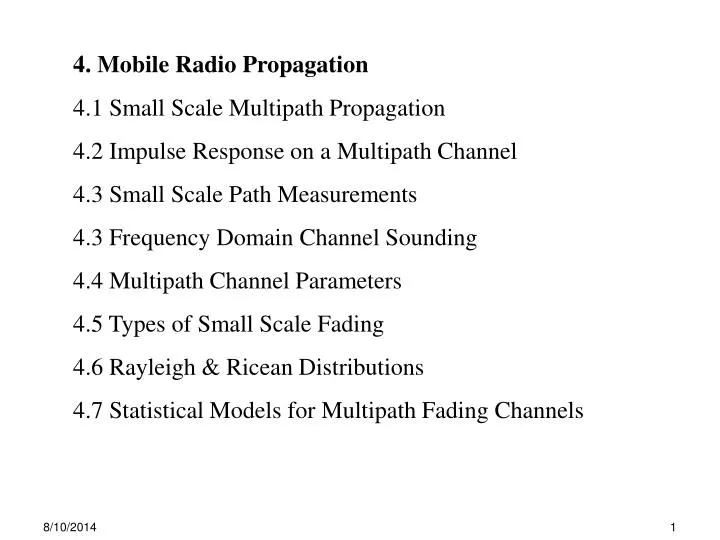
4. mobile radio propagation 4. Mobile Radio Propagation 4.1 Small Scale Multipath Propagation 4.2 Impulse Response on a Multipath Channel 4.3 Small Scale Path Measurements 4.3 Frequency Domain Channel Sounding 4.4 Multipath Channel Parameters 4.5 Types of Small Scale Fading 4.6 Rayleigh & Ricean Distributions 4.7 Statistical Models for Multipath Fading Channels

4. Mobile Radio Propagation – Small Scale Fading - Multipath • Fading: rapid fluctuations in amplitude over short time & distance • antennas radiate electromagnetic (EM) waves over a wide angle • EM waves reflect off of random objects • transmitted signal arrives at a point from many different paths • with different phases • wide variation in phase & amplitude – depending on distribution • large-scale effects are negligible – not distance dependent

d1 d0 d2 t0 ≈t1 t2 Fading • multipath components (MPCs) – reflected EM wave components • if time delayof MPCs ≈ symbol duration then interference (fading) can • result • coherence bandwidth, Bc, is related to channel’s multipath structure • measure of maximum frequency difference between signals with • strongly correlated amplitudes

4.1 Small Scale Multipath Propagation • important effects: • (i) rapid changes in signal strength over small distances & time • intervals • (ii) Doppler shifts on different multipaths  random frequency • modulation • (iii) time dispersion (echoes) caused by multipath small scale MP propagation • Multipath in Urban Areas • NLOS path - mobile antenna height < surrounding structure’s height • even with LOS path  multipath exists • received signal at any point consists of many plane waves with • - randomly distributed amplitudes phases, angles • - components combine vectorially at receiver • - causes distorted or faded signal reception

Characteristics of Fading • Spatial Fading: all objects are stationary – only mobile moves • spatial variations appear as temporal variations at mobile receiver • constructive & destructive effects of multipath in multipath field • moving objects disturb the field – constructively or destructively High Mobility: receiver passes through several fades in a short time Low Mobility: extended time in a deep fade possible Doppler shift: relative mobility between TX & RX  proportional to direction & velocity

(i) multipath propagation and multipath components (MPCs) • presence of objects cause reflection & scattering • dissipates energy in amplitude, phase, time • multiple versions arrive at different times and spatial orientation • causes signal smearing - intersymbol interference (ISI) • (ii) relative speed between Tx-Rx results inDoppler shift – random • frequency modulation • (iii) moving objects: induce time varying Doppler shift on MPCs • if speed of objects > mobile speed  objects dominates fading • otherwise object speed can be ignored • impact also depends on size & shape of objects 4.1.1: Four Factors of Fading

1 0 0.75 - 10 0.5 e e 0.25 - 20 d d PSD (dB) u u t t i i 0 l l p p m m a a - 30 - 0.25 - 0.5 - 40 - 0.75 - 0.4 - 0.2 0 0.2 0.4 2.5 2.5 3.0 3.0 4.0 4.0 4.5 4.5 5.0 5.0 5.5 5.5 6.0 6.0 time Frequency 0.23ns 1 0 0.75 - 10 0.5 4.4GHz 0.25 - 20 PSD (dB) 0 - 30 - 0.25 - 0.5 - 40 - 0.75 - 0.4 - 0.2 0 0.2 0.4 time Frequency (iv) bandwidth of transmitted signal • if signal bandwidth > multipath channel ‘bandwidth’ • - received signal will be distorted • - signal strength won’t fade over a small area – insignificant small • scale fading • if signal bandwidth << physical channel bandwidth • - rapidly changing signal amplitude - fading • - but signal won’t be distorted • signal bandwidth is proportional to 1/symbol duration (width)

4.1.2 Doppler shift S = signal source v = velocity d = distance Y-X on mobiles path of movement t = d/v l = dcos1= vtcos 1 if S is far away, assume 1≈ 2 S l 1 2 X Y d v phase shift:  = (4.1) fd= (4.2) Doppler shift = relative frequency change during t

v S v S • e.g. fc= 1850 MHz   = c/fc = 0.162m • v = 60mph = 28.62 m/s • a. mobile moving directly towards transmitter:  = 0o  cos  = 1 • fd = v/ = 160Hz • f = fc + fd= 1850.00016MHz • b. mobile moving directly away from transmitter •  = 180o  cos  = -1 • fd = -v/ = -160Hz • f = fc + fd= 1849.99984MHz • c. mobile moving  to angle of signal’s arrival •  = 90o cos  = 0 • fd= 0

h(t) x(t) y(t) 4.2 Impulse Response on a Multipath Channel 4.2 impulse response of MP channel • Channel Model used to predict & compare performance of • (i) different communications systems • (ii) different transmission bandwidths for a particular condition • Small Scale Signal Variations are related to RF channels impulse • response • channel impulse response is a wideband channel characterization • contains all information necessary to simulate/analyze any • transmission • similar to concept of transfer function and input/ouput in control • systems

Organization of 4.2: (1) Mobile RF Channel Models (2) Multipath Channels and Delay Spread (3) Channel’s Power Delay Profile 4.2.1 Bandwidth vs Received Power (1) wideband pulsed transmitted RF signal, x(t) (2) Continuous Wave (CW) signal

(1) Mobile RF Channel Models • i. linear time-invariant (LTI) system • MPCs have variablepropagation delays - depending on receiver • location • impulse response of LTI channel is a function of receiver position • and does not depend on time • ii. linear filter with time-varying impulse response • time variation is due to receiver motion • at time t, many waves are arriving - filter’s nature is result of sum • of all amplitudes & delays Channel Classification based only on h(t,) , noise is not considered

h(t,d) y(d,t) x(t) then y(d,t) = x(t) h(d,t) = (4.3) if channel is causal (no output until input is applied) then for t < 0 h(d,t) = 0 and y(d,t) = (4.4) • 1.1 Assume time variation is strictly from receiver motion • v = velocity • d = fixed position between Tx & Rx • let y(d,t) = received signal at position d & time t • h(d,t)= channel impulse response • x(t) = transmitted signal

h(vt,t) y(t) x(t) (4.7) y(t) = then y(vt,t) = (4.6) 1.2 Assume constant v position at any time t is given by d = vt (4.5) since v is constant  received signal y is just a function of t y(t) = x(t) h(vt,t) = x(t) h(d,t) channel model: linear time-varying channel that changes with t & d

y(t) = x(t) h(t,) (4.8) = • 1.3 Assume v is constant over short intervals (distances) and let • x(t) = transmitted bandpass wave form • y(t) = received waveform • h(t,) = impulse response of time varying multipath RF channel • completely characterizes channel • is a function of variables t &  • t represents time variation due to motion •  represents channel multipath delay for fixed t y(t) is the convolution of input signal & channel impulse

i. Bandpass Channel Impulse Response Model h(t, )=Re{hb(t, ) exp(jwct)} x(t) y(t) x(t) = channel input or transmitted signal y(t) = channel output or received signal • Assume (reasonably) that multipath channel is • bandlimited • bandpass h(t,) is equivalently described by its complex baseband impulse responsehb(t,) h(t, ) = Re{hb(t, ) exp(jwct) }

c(t) & r(t) are complex envelope representations of x(t) & y(t) r(t) = c(t)  ½ hb(t, ) (4.9) x(t) = Re{c(t)exp(j2fct)} (4.10) y(t) = Re{r(t)exp(j2fct)}(4.11) c(t) r(t) ½ hb(t, ) ii. Baseband Equivalent Channel Impulse Response Model • use Complex Envelope to represent transmitted & received signals • Complex Envelope properties cause ‘½ ‘ factor in 4.9 • needed to represent passband RF system at baseband • low pass characterization removes high frequency variations from • carrier – makes for easier signal analysis

Average Power of bandpass signal, x(t) is given by (COU93) • overbar denotes • - ensemble average for stochastic signal or • - time average for deterministic signal

Let  = multipath delay axis of impulse response • discretizeinto equaltime-delay segmentsor excess delay bins   0 1 2 3 4 • each bin has time delay width given by •  = i+1 - i • 0 = 1st arriving signal  if 0 = 0  = 1 • i = i· with N total equally spaced components 0 1 2 3 4 • (2) Multipath Channels and Delay Spread • Rx receives a series of replicas of transmitted signal that are attenuated, • time-delayed, phase-shifted MP channel Delay Spread All MPCs received in ith bin are represented as one Resolvable MPC with delayi

Quantization of Delay Bins determines channel’s time delay resolution • model’s useful frequency span = maximum signal bandwidth that • can be analyzed is given as 1 • model’s frequency span = 2 D t e.g. if  = 1ns  maximum signal bandwidth limited to 2GHz • propagation delay from transmitter to receiver is often neglected • by setting excess time delay of 1st MPC = 0 • 0 = 0 • Excess Delay - denoted by i, is the relative delay of ith MPC • relative to 1st arriving component • Maximum Excess Delayof the channel is given by  MAX = N

hb(t, ) t1 t2 t3 0 1 2 3 4 5 6 7 8 9 t0 t0 t1 t2 t3 t • Time-varying Discrete Impulse Response Model for multipath channel • different snapshots of hb(t, ) at times ti

hb(t, ) t t3 (t3) t2 (t2) t1 (t1) t0 time amplitude (t0) 0 1 2 3 4 … N-2 N-1 delayedmultipath components • Time-varying Discrete Impulse Response Model for multipath channel • time = t varies into the page • time delay bins are quantized to widths = 

hb(t,) = (4.12) Baseband Impulse Responseof multipath channel: • N = total possible MPCs (bins) • () = unit impulse function – determines specific multipath bins which have • components at time t & excess delay i • i(t) = excess delay of ith MPC at time t • i(t, ) =real amplitudes of ith MPC at time t • if i(t,) = 0  excess delay bin has no MPC at time t & delay i • 2fci(t)+i(t, ) = all mechanisms for phase shifts of one MPC in ithbin • includes free-space propagation of ith MPC at time t & any additional • phase shifts in channel • often represented as one channel variable: i(t, ) = 2fci(t)+i(t, )

MPC model in a delay bin is affected by choice of  and channel properties (geometry) • for example: • (i) with 1 MPC arriving in a delay bin - amplitude will not fade • significantly over a small area • (ii) with 2 or more unresolveableMPCs arriving in a delay bin • they vectorially combine to yield instantaneous amplitude & phase • of a single MPC model • multipath amplitude in a bin will fade over local area

hb(t,) = (4.13) • Assume channel impulse response is either time invariant or stationary over a small time-scale or distance interval • hb(t,)in (4.12) can be simplified to : i =constant per excess delay bin i= constant per excess delay bin

time invariant channel: i has constant amplitude time variant channel: i has time varying amplitude r(t) = h()= h()= if if r(t)= r(t)=   Pass Band Channel Models • r(t) = s(t)  h(t) + n(t) • r(t) = received signal • s(t) = transmitted signal • h(t) = impulse response of channel • n(t) = AWGN

(3) Channel’s Power Delay Profile(PDP) for small-scale channel model power delay profile • determined by taking spatial average of |hb(t,)|2 over local area • build ensemble PDP by taking several measurements of |hb(t,)|2 • over a local area • each ensemble represents possible small scale channel state • Probing pulse,p(t) is used to ‘sound’ the channel to measure hb(t,) • p(t) approximates delta function p(t)  (t -) (4.14) • if p(t)’s time duration << impulse response of channel (Cox72,75) • p(t)’s bandwidth >> channel bandwidth • p(t) doesn’t need to be deconvolved from received signal, r(t) to • determine relative multipath signal strengths

P() k |hb(t,)|2(4.15) Received Power Delay Profile (PDP) in a local area given by: • P() = single, time-invariant multipath power delay profile • typically derived from many snapshots of |hb(t,)|2averaged • over local area (small scale) • bar represents average over local area • k = gain relating transmit power in p(t) to total power received in • multipath delay profile

4.2.1 Bandwidth vs Received Power 4.2.1 Bandwidth vs Received Power • impulse response of multipath channel is measured in a field using • channel sounding techniques – aka probes • 2 extreme cases of small scale fading in the same channel – show • variation in fading behavior for signals with different bandwidths (1)Wideband pulsed transmitted RF signal, x(t) (2) Continuous Wave (CW) signal

Tbb Max TREP • x(t) = Re{p(t)exp(j2fct)} • - p(t) = periodic baseband pulse train with very narrow pulse width Tbb • - MAX = maximum excess delay in channel • - TREP = pulse period, with TREP >> MAX  wideband pulse p(t) will yield output  hb(t,) (1) Consider wideband pulsed transmitted RF signal, x(t)

for 0  t  Tbb p(t)= p(t) = 0 elsewhere r(t) = r(t) = For all excess delay, i, of interest, assume p(t) is a square pulse with • Low Pass Channel Output, r(t) = hb(t) convolved with p(t) • r(t) will closely approximate channel impulse response, hb(t) (4.16)

e.g. excess delay: let MAX = 40ns and Tbb = 10ns then p(t)= = 4 for 0  t  Tbb, 2 40 / 10 = 0 elsewhere and = = r(t) =

(4.17) |r(t0)|2 = |r(t0)|2 = • Determine Received Power at time t0 measured power = |r(t0)|2 • |r(t0)|2 = energy received in time duration of multipath delay • divided by MAX • found by summing multipath power resolved in channel’s • instantaneous multipath power delay profile, |hb(t,)|2 • using 4.16 we have:

= 0 and if i  j 2.|r(t0)|2 = = = • if all MPCs are resolved by probe p(t)then • 1. the difference between any excess delay components is greater • than the pulse width •  i  j |j - i| > Tbb (4.18)

thusfor wideband probe p(t) with narrow pulse widthTbb • if Tbb < delays between MPCs in the channel  then from 4.18, • total received power at any time is • related to  all powers in individual multipath components • scaled by • - ratio of p(t)’s width & amplitude • - channel’s maximum observed excess delay

E, [PWB]  (4.19) • Practically received power from MPCs is random process • at any time t, each component has randomamplitude & phase • average small scale received power for wideband probe is found • from (4.17) as • E,[]  denotes ensemble average in a local area over all possible • values of i & i • PWB = instantaneous received power from wideband pulse • overbar denotes sample average over local measurement area • - generally measured using multipath measurement equipment

from 4.18 & 4.19: if transmitted signal is able to resolve multipaths then: • small-scale received power =  received power in each MPC • practically, amplitudes of individual MPCs don’t fluctuate widely • in a local area • - received power of wideband p(t) does not fluctuate widely when • receiver moves in a local area • - reduced fading in a local area next slide is continuous wave signal

(2) Continuous Wave (CW) signal • denote complex envelope of CW signal by c(t) = 2 • CW signal transmitted in same multipath channel hb(t,) = • received signal’s instantaneous complex envelop given by phasor sum r(t) = (4.20) • instantaneous received power given by: |r(t)|2 = (4.21)

channel changes as receiver moves in local area (distances  ) • received signal strength varies from fluctuations in i & i • i varies little over local area • i varies greatly due to changes in propagation distance • phase variations causes large fluctuations in r(t) as receiver moves • thus, since r(t) is phasor sum of individual MPCs • instantaneous phase of MPCs cause large fluctuations in r(t) • typifies small-scale fading for CW signals

(4.22) E [PCW] = E [PCW]  (4.23)  (4.24) where rij= path amplitude correlation coefficient defined as: rij = E[i, j] (4.25) average received power over a local area for CW signal is given by: overbar denotes average CW measurements at a mobile receiver in a local area

In a Small-scale Region, if and/or rij= 0  then average received power of CW & wideband signals are equivalent • By comparison of 4.19 & 4.24 this situation can occur when either • (i) multipath phases areiid uniform over [0,2] • iid uniform distribution of  is a reasonable assumption • (iid= identically & independently distributed ) • (ii) path amplitudes are uncorrelated • MPCs traverse differential path lengths that measure 102’s  • MPCs are likely to arrive in random phases • if path phases are dependenton each other  then path amplitudes • are likely to correlated • - mechanisms affecting path phase will likely affect amplitude • - highly unlikely at mobile RF frequencies

thus Received Local Ensemble Average Power of wideband & narrow band signals are equivalent in a small scale region • wideband transmission: transmitted signalbandwidth>> channel • bandwidth • multipath structure is completely resolved by received signal at • any time • received power varies little – individual multipath amplitudes do • not vary rapidly in a local area • narrow bandwidth: baseband signal duration > channel’s excess • delay • multipath is not resolved by received signal • large fluctuations (fading) occurs at receiver due to phase shifts of • many unresolved MPCs

indoor RF channel measurements • assume measurement track = 5 (0.375m) • transmit CW signal and probing pulse signal • (i) CW transmitterfc = 4GHz  = 0.075m (7.5cm) • - CW signal undergoes rapid fades with local mobility • (ii) wideband probing pulse  Tbb = 10ns • - wideband measurements change little over measurement track • Local Average Received Powers of Either are Nearly Equal ! indoor RF channel measurements

(1) Narrow Band CW Signal  =7.5cm fc= 4GHz 10dB (2) Wideband Pulse, Tbb = 10ns 5  1.25ns (0.375m) (1/Tbb = 100MHz) Relative Received Power 0.00 0.25 0.50 0.75 1.00 12 14 16 ’s 0 50 100 150 200 250 Excess Delay (ns)

e.g. 4.2: discrete channel impulse response – used to model example 4.2 (a) Width of Excess Delay Bin  = MAX/N (b) Maximum Bandwidth Accurately represented = 2/ • Let MAX= max excess delay N • N = 64 multipath bins &  = MAX/64

v 1 2 • e.g. 4.3 • mobile traveling at v = 10m/s • fc = 1GHz   = c/fc = 0.3m • 2 multipath components received with properties given below example 4.3 • Mobile moves directly towards 1 & directly away from 2 • a. find narrowband instantaneous power at intervals = 0.1s & 0.5s • b. find average narrowband power over interval 0.1s-0.5s • c. compare average narrowband & wideband received power over • interval 0.1-0.5s

i = (i) instantaneous power given by: |r(t)|2 = (ii) phase: mobile moves - phase of 2 components changes in opposite directions |r(t)|2 = spatial interval = v ·t at t = 0  phase of both components, i= 0 and instantaneous power given by:

instantaneous power, |r(t)|2 = the phase of each component given by 2vt/ at t = 0.1s • 1 = 2(10m/s)(0.1s)/0.3 = 20.94 rad •  20.94 rad – (3·2 )rad = 2.09rad = 120o 2 = 2(-10m/s)(0.1s)/0.3 = -20.94rad = -120o |r(t)|2 = 78pW

t 1 2 instantaneous power |r(t)|2 phase i = 0 0o 0o 291pW 0.1 120o -120o 78.2pW 0.2 240o -240o 81.5pW instantaneous power |r(t)|2 = 0.3 360o -360o 291pW 0.4 120o -120o 78.2pW 0.5 240o -240o 81.5pW 1 = 2(10m/s)(t)/0.3 2 = 2(-10m/s)(t)/0.3 phase and instantaneous power over interval 0s - 0.5s

Average Wideband Received Power E, [PWB]  = 100pW + 50pW = 150pW • Average Narrowband Received Power • 0.167 [2(291)pW + 2(81.5) + 2(72.2)] = 150.23pW

4. mobile radio propagation