Download
1 / 33
330 likes | 521 Vues
Beyond delta-N formalism. Atsushi Naruko Yukawa Institute Theoretical Physics, Kyoto In collaboration with Yuichi Takamizu ( Waseda ) and Misao Sasaki (YITP). The contents of my talk. 1. Introduction and Motivation 2. Gradient expansion and delta-N formalism

E N D
Beyond delta-N formalism Atsushi Naruko Yukawa Institute Theoretical Physics, Kyoto In collaboration with Yuichi Takamizu (Waseda) and MisaoSasaki (YITP)
The contents of my talk 1.Introduction and Motivation 2.Gradient expansion and delta-N formalism 3.Beyond delta-N formalism
Introduction • Inflationis one of the most promising candidates as the generation mechanism of primordial fluctuations. • We have hundreds or thousands of inflation models. →we have to discriminate those models • Non-Gaussianity in CMB will have the key of this puzzle. • In order to calculate the NG correctly, we have to go to thesecond order perturbation theory, but …
Evolution of fluctuation Gradient expansion Perturbation theory Concentrating on the evolution of fluctuations on large scales, we don’t necessarily have to solve complicated pertur. Eq.
Gradient expansion approach • In GE, equations are expanded in powers of spatial gradients. →Although it is only applicable to superhorizon evolution, full nonlinear effects are taken into account. • At the lowest order in GE (neglect all spatial gradients), = lowest order Eq. Background Eq. • Just by solving background equations, we can calculate curvature perturbations and NG in them. :delta-N formalism (difference of e-fold) • Don’t we have to care about spatial gradient terms ?
Slow-roll violation • If slow-roll violation occured, we cannot neglect gradientterms. Power spectrum of curvature pert. Slow-roll violation Leach, et al (PRD, 2001) wave number • Since slow-roll violation may naturally occur in multi-field inflation models, we have to take into account gradient terms more seriously in multi-field case.
Goal Our goal is to give the general formalism for solving the higher order terms in (spatial) gradient expansion, which can be applied to the case of multi-field.
Gradient expansion approach • On superhorizon scales, gradient expansion will bevalid. →We expand Equations in powers of spatial gradients : ε • We express the metric in ADM form • We decompose spatial metric gijand extrinsic curvature Kijinto a(t) : fiducial “B.G.” Ψ 〜 R : curvature perturbation traceless
Lowest-order in gradient expansion • After expanding Einstein equations, lowest-order equations are lowest-order eq. background eq. →The structure of lowest-order eq is same as that of B.G. eq with identifications, and ! changing t by τ lowest-order sol. background sol.
delta-N formalism • We define the non-linear e-folding number and delta-N. Ψ E • Choose slicing such that initial : flat & final : uniform energy Efinal E const. flat flat Einitial flat delta-N gives the final curvature perturbation
Gradient expansion approach delta-N Beyond delta-N Gradient expansion Perturbation theory
towards “Beyond delta-N” • At the next order in gradient expansion, we need to evaluate spatial gradient terms. • Since those gradient terms are given by the spatial derivative of lowest-order solutions, we can easily integrate them… • Once spatial gradient appeared in equation, we cannot use “τ” as time coordinate which depends on xi because integrable condition is not satisfied. →we cannot freely choose time coordinate (gauge) !!
Beyond delta-N • We usually use e-folding number(not t) as time coordinate. →We chooseuniform Ngauge and use N as time coordinate. • Form the gauge transformation δN: uniform N → uniform E, we can evaluate the curvature perturbation . E const. lowest order next order flat
Summary • We gave the formalism, “Beyond delta-N formalism”, to calculatespatial gradient terms in gradient expansion. • If you have background solutions, you can calculate the correction of “delta-N formalism” with this formalism just by calculating the “delta-N”.
FLRW universe • For simplicity, we focus on single scalar field inflation. • Background spacetime: flat FLRW universe Friedmann equation :
Linear perturbation • We define the scalar-type perturbation of metric as (0, 0) : (0, i) : trace : traceless :
Linear perturbation : J = 0 • We take the comoving gauge = uniform scalar field gauge. • Combining four equations, we can derive the master equation. • On super horizon scales, Rc become constant. and
Einstein equations in J = 0 • Original Einstein equations in J = 0 gauge are (0, 0) : (0, i) : trace : traceless :
Rc = a δφflat • We can quantize the perturbation with • u is the perturbation of scalar field on R = 0 slice. →quantization is done on flat (R = 0) slice. →perturbations at horizon crossing which give the initial conditions for ▽ expansion are given by fluctuations on flat slice.
Curvature perturbation ? • We parameterised the spatial metric as traceless linearlise • In the linear perturbation, we parametrised the spatial metric as R : curvature perturbation • Strictly speaking, Ψ is not the curvature perturbation. →On SH scales, E become constant and we can set E = 0. →Ψ can be regarded as curvature perturbation at lowest-order in ▽ expansion.
Shear and curvature perturbation • Once we take into account spatial gradient terms, shear (σgor Aij) will be sourced by them and evolve. →we have to solve the evolution ofE. • At the next order in gradient expansion, Ψ is given by “delta-N” like calculation. In addition, we need to evaluate E.
delta-N formalism 1 • We define the non-linear e-folding number • Curvature perturbation is given by the difference of “N” flat N flat xi = const.
delta-N formalism 2 • Choose slicing such that initial: flat& final : uniform energy φ Ψ E const. E const. flat E const. flat flat delta-N gives the final curvature perturbation
Beyond delta-N • We usually use e-folding number(not t) as time coordinate. →We chooseuniform N slicing and use N as time coordinate. • Combining equations, you will get the following equation for φ.
Beyond delta-N 2 • We compute “delta N” from the solution of scalar field. φ com. = com. flat
Beyond delta-N 3 • We extend the formalism to multi-field case. • As a final slice, we choose uniform E or uniform K slice since we cannot take “comoving slice”. • We can compute “delta N” form the solution of E, K. @ lowest order
Question How can we calculate the correction of delta-N formalism ?
Answer To calculate the cor. of delta-N, all you have to do is calculate “delta-N”.