Download
1 / 32
320 likes | 424 Vues
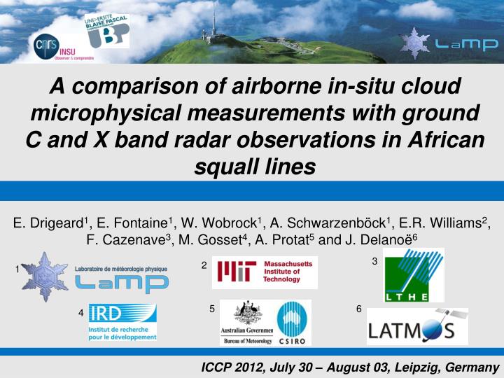
A comparison of airborne in-situ cloud microphysical measurements with ground C and X band radar observations in African squall lines. E. Drigeard 1 , E. Fontaine 1 , W. Wobrock 1 , A. Schwarzenböck 1 , E.R. Williams 2 , F. Cazenave 3 , M. Gosset 4 , A. Protat 5 and J. Delanoë 6. 3. 2. 1.

E N D
A comparison of airborne in-situ cloud microphysical measurements with ground C and X band radar observations in African squall lines E. Drigeard1, E. Fontaine1, W. Wobrock1, A. Schwarzenböck1, E.R. Williams2, F. Cazenave3, M. Gosset4, A. Protat5 and J. Delanoë6 3 2 1 5 6 4 ICCP 2012, July 30 – August 03, Leipzig, Germany
French-Indian satellite (launched on the 11/10/12) To improve our knowledge of the processes linked to the tropical convection and precipitation 2 ground validation campaigns (Niger & Maldives) Aircraft measurements with the French Falcon 20 (CIP, PIP, 2DS probes, cloud radar RASTA)
French-Indian satellite (launched on the 11/10/12) To improve our knowledge of the processes linked to the tropical convection and precipitation 2 ground validation campaigns (Niger & Maldives) Aircraft measurements with the French Falcon 20 (CIP, PIP, 2DS probes, cloud radar RASTA) 2 ground radars : MIT & Xport Objective : comparing ground based radar reflectivity with those calculated from in-situ microphysical observations
Volumetric protocol : • 3D spatial distribution of the reflectivity every 12 minutes • Elevations : • - Xport : 12 angles • from 2 to 45° • - MIT : 15 angles • from 2 to 24°
MIT radar : On the Niamey airport C-band (5.5 GHz) Range of 150km Xport radar : 30 km SE of the airport X-band (9.4 GHz) Range of 135km + MIT radar ΔXport radar 90 km • To compare radar data and in-situ observations : • Co-localization of the 2 ground radars data • and the aircraft position
8 250 m 7 5 250 m 4 6 1 3 2 1- 7° 1° Radar • Use of all scans collected during a observationnal period • Steady state hypothesis of the reflectivity field during this period (increasing the vertical resolution) • Spatial interpolation (Inverse Distance Weighting) using 8 observation points
Calculated RHI (15 scans) Measured RHI (300 scans) • Comparison of observed and calculated RHI scans for the MIT radar • Differences increase with distance (deterioration of the vertical resolution of the volumetric data) • Statistical analysis : • standard deviation = 3dBZ ± 3dBZ
Good agreement between co-localized MIT reflectivity and airborne radar RASTA Very similar pattern for the airborne and the ground observation
In-situ probes (PIP, CIP, 2DS) show cloud particles from 50µm to 5mm. The cloud particles have irregular shapes (graupel, aggregate) To calculate the equivalent reflectivity Ze, a power mass law m=αDβ is applied: Example for number distribution averaged during 10s during the flight #20
In-situ probes (PIP, CIP, 2DS) show cloud particles from 50µm to 5mm. The cloud particles have irregular shapes (graupel, aggregate) To calculate the equivalent reflectivity Ze, a power mass law m=αDβ is applied: α is determined by matching the reflectivity calculated by Mie theory with measurements of the cloud radar RASTA at 95GHz 0.001 < α < 0.1; and β = 2.1 The mass law obtained in this way is applied again to calculate the reflectivity of the precipitation radars MIT and Xport (using Rayleigh approximation)
- Calculated reflectivity is in good agreement with observations of both ground radars - Best results in regions where aircraft < 8000 m and range < 80 km
Some periods with differences between signals • Statistically :
Reflectivity observed by precipitation radar can be recalculated from in-situ cloud microphysical measurements, if a mass-diameter relationship in a form of m=αDβ is applied (instead of m~D3) Limits : mixte phase clouds and predominantly cold clouds (in the levels from -5 to -30°C) where reflectivity prevails from 15 to 35 dBZ. Perspectives: on-going work on the differences observed between both ground based radars improving satellite retrieval processes in the Megha-Tropiques context
Contexte MT1 + MIT radar Δ Xport radar • 3 vols étudiés en particulier • Vol 18 : 13/08/2010 après-midi • Vol 20 : 17/08/2010 nuit • Vol 23 : 26/08/2010 matin • 2 radars au sol (décalés de 30km) : • MIT : 593*360*15 = 3 202 200 points / fichier • XPORT : 677*360*12 = 2 924 640 points / fichier • Portée MIT : 150km • Elévation max = 24° • Portée XPORT : 135km 80km • Elévation max = 45°
Constat : fortes différences entre les PDF MIT et XPORT • Sur ces figures : • XPORT sur sa propre grille, sur la durée totale du vol, avec R < 80km & alti<12km • MIT non corrigé sur sa propre grille, sur la durée totale du vol, avec R/XPORT < 80km & alti<12km Besoin de corriger les données MIT 25 238 923 val 16 779 568 val 10 773 505 val 10 898 711 val 11 166 915 val 10 814 451 val
Intercomparaison des deux radars • Pour déterminer la correction à appliquer : étude du rapport ZXPORT/ZMIT • Problème : deux grilles distinctes pour les deux jeux de données • Intercomparaison des deux radars avec code de colocalisation De la même façon qu’on a colocalisé les données radars sol sur la trajectoire de l’avion Falcon, on colocalise les données de l’un des deux radars sur la grille de l’autre (et inversement) • Utilisation de la grille XPORT comme référence interpolation des mesures MIT aux coordonnées (x, y, z, t) du XPORT • Utilisation de la grille MIT comme référence interpolation des mesures Xport aux coordonnées (x, y, z, t) du MIT • Méthodologie : • Transformer les coordonnées d’observation (range, azimuth, elevation) du radar de référence dans un repère géographique : latitude, longitude, altitude création d’une « trajectoire d’avion » virtuelle • Interpoler les observations du 2nd radar aux points du radar de référence • Sélection des données telles que : ZXPORT & ZMIT > -5dBZ & alti < 12km & dist/XPORT<80km • Finalement : entre 10 et 25 millions de couples de valeurs pour chaque vol
Facteur de correction • Étude du rapport ZXPORT/ZMIT (en mm6/m3) pour les données sélectionnées : • 5.5km < alti < 12km • R/XPORT < 80km • Résultats : • facteur de correction moyen pour le vol 18 = 7.07 (écart-type = 5.07) • facteur de correction moyen pour le vol 20 = 5.39 (écart-type = 4.66) • facteur de correction moyen pour le vol 23 = 4.82 (écart-type = 4.45) 10 773 505 val 10 898 711 val 13 361 414 val 11 166 915 val 10 814 451 val 13 251 095 val 25 238 923 val 16 779 568 val 20 426 838 val
Facteur de correction • Étude du rapport ZXPORT/ZMIT (en mm6/m3) pour les données sélectionnées : • 5.5km < alti < 12km • R/XPORT < 80km • Résultats : • facteur de correction moyen pour le vol 18 = 7.07 (écart-type = 5.07) • facteur de correction moyen pour le vol 20 = 5.39 (écart-type = 4.66) • facteur de correction moyen pour le vol 23 = 4.82 (écart-type = 4.45) 10 773 505 val 13 361 414 val 25 238 923 val 20 426 838 val 11 166 915 val 13 251 095 val 11 166 915 val 10 814 451 val 13 251 095 val 25 238 923 val 16 779 568 val 20 426 838 val
20 381 012 val 16 779 568 val 20 426 838 val 13 155 011 val 10 898 711 val 13 361 414 val 12 982 448 val 10 814 451 val 13 251 095 val
13 155 011 val 13 361 414 val 12 982 448 val 13 251 095 val 20 381 012 val 20 426 838 val Bonne concordance entre les PDF en particulier pour les fortes réflectivités caractéristiques des fortes précipitations
Sélection des « meilleures données » : • Différence temporelle entre les mesures de chaque radar < 30 sec • Différence verticale < 5% de l’altitude de la mesure interpolée • Filtre très important des données : < 1% de données restantes • Validation des jeux de données et de la méthode de colocalisation 3 609 val 3 680 val 6 020 val 5 936 val 2 699 val 2 785 val
Contexte MT2 DYNAMO • 2 vols étudiés en particulier • Vol 45 : 27/11/2011 matin • Vol 46 : 27/11/2010 après-midi • 2 radars au sol (distants de 2.5km) : • SPOL (2.80GHz) : 979*360*8 = 2 819 520 points / fichier • 5 min de mesures toutes les 15 min • SMART (5.63GHz) : 1499*360*26 = 14 030 640 points / fichier • 7.5 min de mesures toutes les 10 min
Contexte MT2 DYNAMO • 2 vols étudiés en particulier • Vol 45 : 27/11/2011 matin • Vol 46 : 27/11/2010 après-midi • 2 radars au sol (distants de 2.5km) : • SPOL (2.80GHz) : 979*360*8 = 2 819 520 points / fichier • 5 min de mesures toutes les 15 min • SMART (5.63GHz) : 1499*360*26 = 14 030 640 points / fichier • 7.5 min de mesures toutes les 10 min • Portée SPOL : 147km • Elévation max = 11° • Portée SMART :150km • Elévation max = 33° Radar SPOL Radar SMART
Comparaison des données • Sur ces figures : • SPOL sur sa propre grille, sur la durée totale du vol, avec R < 120km & alti<12km • SMART sur sa propre grille, sur la durée du vol, avec R < 120km & alti<12km 6 745 230 val 9 574 265 val 4 554 910 val 12 711 956 val
Intercomparaison des deux radars • Même technique que pour MT1 : colocalisation de l’un des deux radars sur la grille de l’autre 10 868 439 val 12 711 956 val 4 869 756 val 9 574 264 val