Download
1 / 88
880 likes | 1.01k Vues
Presentation on Row Reduction Techniques. Presented By : Name: Amit Grover Email : grover@usc.edu. Topics covered in this presentation. What is Row Reduction. What are the reasons for doing Row Reduction What are state variables and external inputs.

E N D
Presentation on Row Reduction Techniques Presented By : Name: Amit Grover Email : grover@usc.edu
Topics covered in this presentation • What is Row Reduction. • What are the reasons for doing Row Reduction • What are state variables and external inputs. • Algorithms used for row reduction • For completely specified state machines. • Pairchart • For incompletely specified state machines • Pairchart • Skill algorithm • Bargain hunter • MEU Method • Applications
Definition • Given a sequential machine, our aim is to find the finite state machine which have same behavior as the given machine but has reduced states.
Advantages of Row Reduction • Cost Reduction • We know Flip Flops used as memory elements are costly and each time a new state is added to the machine we are adding new memory element to it. • Addition of this new element needs space in the logic circuits and thus increases the size of the logic circuit • Adds cost the logic circuit • These additions adds significant amount of cost to the Logic circuit and we don’t want that, so our aim is to reduce the cost as much as possible without effecting the functionality of the logic circuit.
State Variables and External Inputs. External Inputs 00 01 11 10 1 2 3 4 State Variables
Completely Specified Machines. • A machine which has no don’t cares in its table is called a completely specified state machine (CSSM). • Let’s see an example to find out what do we mean by having no don’t cares.
Completely Specified State Machine(CSSM) External Inputs A B 1 2 3 4 5 6 State Variables No don’t cares
Incompletely Specified State Machines (ISSM) • Those machines whose next state or output has don’t care is called as ISSM. • Let’s see with diagram what is ISSM.
Incompletely Specified State Machine (ISSM) External Inputs A B 1 2 3 4 5 6 State Variables
Completely Specified Machine • Pairchart Algorithm. • Things given to you. • Flow table. • Aim is to reduce the number of rows as much as possible. Steps Involved • Draw Pairchart. • Check for output Incompatibility and cross out all those which are incompatible. • Check for next state incompatibilities and cross out all those which are incompatibles. • Repeat step iii till you get no next state incompatible state. !!These things will be more clear with a example which follows..
Given CSSM A B 1 2 3 4 5 6 Figure 1
How to read CSSM A B 1 2 3 4 5 6 • If you are in State 1 and input is A you go to State 2 with output 0. • If you are in State 1 and input is B you go to State 3 with output 1. • If you are in State 3 and input is A you go to State 2 with output 0. • And so on……
Step 1 for Pairchart Algorithm • Look at the Maximum Number of States you have. • In our case it is 6. (Refer previous given CSSM). • Now write the States from 1->6 horizontally in increasing order and from Top to Bottom in increasing order. • This Step is shown in next slide….
Implementation of Step 1 of Pairchart Algorithm 1 2 3 4 5 6 Increasing Order 1 2 3 4 5 6 Increasing Order
Step 2 of Pair Chart Algorithm • We can remove half of the pairchart (diagonally) because it is symmetric along the diagonal. • So we are effectively duplicating along the diagonal. • So after removing half of the portion from diagonal, we get something like this.(shown in next slide).
Implementation of Step 2 of Pairchart Algorithm 1 2 3 4 5 6 Increasing Order Cutting from diagonal 1 2 3 4 5 6 Increasing Order
A B Figure2 1 2 1 2 3 4 5 6 3 4 5 6 Increasing Order 1 2 3 4 5 6 Increasing Order
Step 3 of Pairchart Algorithm • Let’s start filling the Table in Figure 2. • Output Compatibility • We will take one column at a time and will check if it is output compatible with each and every other state. • Question comes what is output compatibility?? • State 1 is Output Compatible with State 2 iff for same input both gives same Output. • Refer to next slide for better explanation..
Column 1 A B • Check if 1 is output compatible • with 2 for both input A and B 1 Answer: No. For same Input A or B State 1 and State 2 has different output. 2 1 2 3 4 5 6 3 X 4 • So we put a cross • in block at the inter • section of 1 and 2. 5 6 1 2 3 4 5 6
Column 1 A B • check if 1 is output compatible • with 3 for both input A and B 1 2 1 2 3 4 5 6 Answer: Yes. For same Input A and B State 1 and State 3 has same output. 3 X 4 • So we don’t do • anything with the • block at the inter • section of 1 and 3. 5 6 1 2 3 4 5 6
A B 1 Similarly we will fill for all the blocks 2 1 2 3 4 5 6 3 X 4 X 5 X X 6 X X X X X 1 2 3 4 5 6
Pairchart Algorithm continued… • Refer to given flow table and take one column at a time in the pairchart and fill each block in that column (excluding those blocks which are having ‘X’ sign) with, where the state representing that column will go when input A and B is given.. Refer to next slide for better explanation.
A B Taking Column represented by state 1 - From pairchart, state 1 goes to state 2 with input A and to state 3 with input B. 1 2 1 2 3 4 5 6 - So we will write 2 and 3 in each block in column 1 and Row 1 as shown.. 3 X 4 3 2 X 5 X X 6 3 2 X X X X X 1 2 3 4 5 6
Pairchart algorithm continued.. • We will continue with all the rows and column and what we get is shown in next slide… • Let’s see how that will look like.
A B Taking next Column represented by state 2 - From pairchart, state 2 goes to state 4 with input A and to state 1 with input B. 1 2 1 2 3 4 5 6 - So we will write 4 and 1 in each block in column 2 and Row 2 (if no ‘X’) as shown.. 3 X 4 3 2 X 5 4 1 X X 6 3 2 X X 4 1 X X X 1 2 3 4 5 6
A B Taking next Column represented by state 3 - State 3 goes to 2 and 1 so we write it in column 3 and also in row 3 -> 2 and 1 1 2 1 2 3 4 5 6 3 X - So we will write 2 and 1 in each block in column 2 and Row 2 (if no ‘X’) as shown.. 4 3 2 X 5 2 1 4 1 X X 6 3 2 2 1 X X 4 1 X X X 1 2 3 4 5 6
A B Lets fill the whole table accordingly 1 2 1 2 3 4 5 6 3 X 4 3 2 X 5 2 1 4 1 X X 6 3 6 3 2 2 1 X X 6 5 6 5 4 1 3 6 X X X 4 5 4 5 1 2 3 4 5 6
Pairchart Algorithm continued.. • So after filling out all the blocks in the pairchart what next… • We need to check each and every block and see if that block is going to some other block which has a ‘X’. (Next State Compatibility) • If Yes then we cross this block. • Else keep moving and check for other states. • Let’s see how it looks like.
Column 1 - Check each block in column 1 for e.g block at the intersection of 1 and 3. A B 1 2 Check Row 2 Column 2 and vice versa.. 2 = 2, so it is okay.Reason is on Slide 17 1 2 3 4 5 6 3 X 4 Check Row 1 and Column 3 or vice versa. In this case, (3,1) references itself, and is not yet X’d, so it is okay. 3 2 X 5 2 1 4 1 X X 6 3 6 3 2 2 1 X X 6 5 6 5 4 1 3 6 X X X 4 5 4 5 1 2 3 4 5 6
A B Column 1 continue…. - Checking next block in column 1 i.e block at the intersection of 1 and 5. 1 2 1 2 3 4 5 6 Check Row 2 Column 6. It does not have a ‘X’. So Okay 3 X 4 Check Row 3 and Column 5 It does not have a ‘X’. So Okay 3 2 X 5 2 1 4 1 X X 6 3 6 3 2 2 1 X X 6 5 6 5 4 1 3 6 X X X 4 5 4 5 1 2 3 4 5 6
A B Column 2 - Check each block in column 2 for e g block at the intersection of 2 and 4. 1 2 Check Row 4 Column 3 and vice versa It has a Cross So Mark This block with ‘X’ Column 3 Row 4. No Need to check this block further. 1 2 3 4 5 6 3 X 4 3 2 X 5 2 1 X 4 1 X X 6 3 6 3 2 2 1 X X 6 5 6 5 4 1 3 6 X X X 4 5 4 5 1 2 3 4 5 6
A B 1 Let’s fill the Whole Pairchart 2 1 2 3 4 5 6 3 X 4 3 2 X 5 2 1 4 1 x X X 6 3 6 3 2 2 1 X X 6 5 6 5 4 1 X 3 6 X X X 4 5 4 5 1 2 3 4 5 6
Pairchart Algorithm continued.. • If you understand everything till this point then assume that you understand most of this algorithm. • There is one last step still left for this algorithm. • Guess what it can be… • Remember what was our aim!!! • To reduce the number of states required to represent the same machine.
Pairchart Algorithm continued.. • It ‘s very easy.. • Draw the graph and link all those states which are compatible to each other with the help of pairchart. • Let’s see how it looks like…
3 Refer Pairchart on slide 35 1 -> Look at column 1 1 is compatible with 3 and 5 5 -> Look at column 2 2 is compatible with 6 2 -> Look at column 3 3 is compatible with 5 6 -> Look at column 4 4 is compatible with none 4 -> Look at column 5 5 is compatible with none ->Look at column 1 6 is compatible with none
Pairchart Algorithm continued.. • Now we need to build up the largest possible circle which covers as much states as possible. • It shows that 135 , 24 and 3 are the states required to represent the same machine.. • So let’s see how the new state machine looks like..
Pairchart Algorithm continued.. 3 1 4 5 2 6
Pairchart Algorithm continued.. New State Assignment A B 135 26 A B 4 1 2 • Refer to our original table and see where State • (1 3 5) go for Input A . • eg in our case it goes to 2 and 6 with output 0. • and for input B it goes to 135. 3 4 - Similarly we will do for 26 and 4. Note : - For 4 we have 3 but there is no state as 3 but 3 is covered by 135 and thus we will write 135,1. Repeat for Input B. 5 6
Review of what we did till now • Till Now we talked about • What State Reduction is.. • We talked about Algorithm which can help us in reducing the rows to reduce the cost of the machine for a given CSSM.. • What next ??? • Now we will talk about ISSM machines and algorithms used for it… • If you really understood till this point it won’t be difficult to understand the rest of stuff..
ISSM Algorithm • ISSM Algorithm is continuation of CSSM pairchart algorithm.. • But there are some more additional algorithms.. • Steps • Pairchart (we already discussed) • Skill algorithm( To get MC’s (Maximum Compatibility Sets) • Bargain Hunter Algorithm. • MEU
ISSM - Pairchart • Since we had talked about Pairchart, I will skip the details and will proceed further.. • But one thing to keep in mind is that in ISSM we have don’t cares and in the pairchart where ever we encounter don’t cares we write don’t cares directly.. • Example is shown in the next slide.
ISSM: Pairchart Algorithm C A B Given: 1 2 3 4 5 6 7 8
After Multiple Passes (Already discussed already) We come to final Table 1 2 3 Shows that 2&3 state is compatible to each other 4 5 1 2 3 4 5 6 6 X 7 X 8 X X X X X X 7 X X 8 X X X X X X X 1 2 3 4 5 6 8 7
Skill Algorithm • This algorithms helps us to get minimal covering machine for ISSM. • This algorithms gives the MC’s (Maximum Compatibility. • Let’s see how it works…
Skill Algorithm Continued… • It consists of different columns • Column K will consists of all the states we have in decreasing order. • Column Sk will contain all those states which are compatible with state in K (We have to refer or pairchart for that). • We compare column Sk and L’ and concatenate state in column K with states which are common to Sk and L’. • Compare Column L’ and states in previous row and its L column and find out all those states which are not covered by each other. • Next slide will make these points much clear..
Skill Algorithm Continue.. Refer Pairchart for State 8 in Column 8 MC’s 8 is not compatible with any one so right NULL in Sk and L’ and 8 in L.
Skill Algorithm Continued.. Refer Pairchart for State 7 in Column 7 7 is not compatible with any one so.. Sk will have NULL. Concatenate 7 with states which Intersects. In this case nothing intersect so Put just 7 in L’ Nothing covers each other so MC’s Look for states which intersect
Skill Algorithm Continued.. Refer Pairchart for State 6 in Column 6 6 is compatible with 7 so.. Sk will have 7. 67 covers 6 and 7 But not 8 so 67,8 in L Concatenate 6 with states which intersects. In this case 7 intersects so It would be 67 in L’ But 7 doesnot intersect with 8 so we will write 6 also in L’ MC’s Look for states which intersect