Download
1 / 31
310 likes | 461 Vues
Propagation of galactic cosmic rays and Jovian electrons in the heliosphere. R. B. McKibben Department of Physics and Space Science Center, Institute for the Study of Earth, Oceans, and Space University of New Hampshire Durham, NH, USA.

E N D
Propagation of galactic cosmic rays and Jovian electrons in the heliosphere R. B. McKibben Department of Physics and Space Science Center, Institute for the Study of Earth, Oceans, and Space University of New Hampshire Durham, NH, USA 1
Propagation of galactic cosmic rays, solar energetic particles, and Jovian electrons in the heliosphere R. B. McKibben Department of Physics and Space Science Center, Institute for the Study of Earth, Oceans, and Space University of New Hampshire Durham, NH, USA 2
First Serious Discussion of Interplanetary Propagation of Energetic Charged Particles:February 1956 Flare(Meyer, Parker, and Simpson, Phys. Rev., 102, 1648, 1956) • Fast rise of intensity suggested direct propagation (i.e. little scattering) of the flare particles between the Sun and the Earth • Slow decay suggested diffusive escape through some sort of scattering region mainly outside the orbit of Earth - what we know today as the heliosphere. Suggested Structure of Interplanetary Space:The First Sketch of the Heliosphere Neutron Monitor Intensity 3
Guidance by interplanetary field lines Diffusion Parallel to Field Perpendicular to Field Convection by Solar Wind Adiabatic Deceleration Gradient and Curvature Drifts in the Interplanetary Field Random walk of field lines Field aligned flows during onset of solar particle events Jovian electron seasons at 1 AU Dissemination of SEP fluxes Rapid onsets/slow decay, backscatter and isotropization of SEP intensities Multi-spacecraft common decays of SEP intensities - “Reservoir Effect” Diurnal Anisotropies, Compton-Getting anisotropies J = A*T Spectra at Low Energies Charge-sign dependence of solar modulation Alternating broad/narrow intensity profiles of nuclei and electrons near solar minimum Flux dropouts in impulsive SEP events,Jovian electron “Jets” Propagation Processes for Energetic Charged Particles in the HeliosphereProcessSample Evidence 4
So What’s the Problem? • Each component of propagation is supported by observational evidence, and each fits well into an overall theory first laid out by Parker (1965). The problem should be solved. • However -- diffusion coefficients continue to present a problem. • There is strong observational evidence that particles both • Propagate efficiently along and are strongly guided by the interplanetary magnetic field lines and also • Propagate efficiently across the mean magnetic field. • Diffusion coefficients parallel and perpendicular to the field can not be specified independently. • Scattering events that produce cross-field diffusion also affect parallel propagation, and vice-versa. • There is an inverse relation between speed of radial diffusion and speed of cross-field diffusion. • It has proven very difficult for theory to reproduce both the parallel and perpendicular propagation rates required by observations. • Do processes other than simple scattering enhance perpendicular propagation? Can observations, which exposed the problem in the first place, also provide clues to its solution? 5
NASA/ESA Ulysses Mission: An ideal probe of propagation processes in the inner heliosphere • Ulysses’ orbit was inclined ~80° to the ecliptic between 1.2 and 5.4 AU • Sampled all latitudes twice per orbit • Sampled all longitudinal intervals wrt near-Earth spacecraft at least once per year • Sampled all radial intervals between 0.2 and 4.4 AU wrt near-Earth spacecraft twice per orbit • Made 2 flybys of Jupiter: 1992 - a few Rj 2004 - 0.8 AU • Completed nearly 3 orbits of the Sun between 1990 and 2009, passing over the Sun’s polar regions 3 times 1994-95 Solar Minimum (A+) 2000-01 Solar Maximum (mixed polarity) 2007-08 Solar Minimum (A-) 6
Ulysses Discovery: Solar Wind Speed and Interplanetary Magnetic Field Structure As a Function of the Solar Cycle Solar Minimum 1994-95 Solar Maximum 2000-01 • At solar minimum, most of the heliosphere is filled with smooth, fast solar wind and monopolar magnetic field lines originating from the polar coronal holes. Mixed field polarities and slow solar wind are mostly confined to a low latitude belt. • There are three different sources (N & S Poles and equatorial) for solar wind, with relatively clean interfaces between them. • At solar maximum, mixed magnetic field polarities and fast and slow solar wind speeds are found at all latitudes. • Chaos reigns. 7
Solar Cycle Modulation over the Ulysses Mission • Daily average intensity/flux records of cosmic rays, with SEP events removed, from the Ulysses COSPIN HET • Left scale: >92 MeV protons and • Right scale: ~35-70 MeV/n He • Daily average solar wind speeds measured by the SWOOPS instrument on Ulysses • Note steady fast solar wind flow from solar polar coronal holes at high latitudes during low solar activity • Ulysses heliographic latitude superposed on the maximum N and S latitudes of the Classic Model Heliospheric Current Sheet, dividing N from S magnetic polarities in the solar wind - as calculated by the WSO. • Light blue bands indicate Ulysses fast latitude scans • Full scan of latitude from 80°s to 80°N in ~ 1 year, a time short compared to the modulation time scale 8
Solar Cycle Modulation over the Ulysses Mission • Wind and field lines in the fast polar solar wind have different origin than field lines in the slow equatorial wind • The transition from fast polar flow to slow equatorial flow correlates well with Ulysses rising above the current sheet region. • Changes of the solar wind speed by a factor of 2 should dramatically change • the spiral angle of the magnetic field • the convection rate • the rate of adiabatic deceleration • the gradient and curvature drift velocity, and • the length of the field line to the heliospheric boundary. All are important for modulation. • The intensities show almost no variation in response to the transitions from polar to equatorial flow. • Higher detail shows modest (of order 10%) intensity variations in quasi-periodic transitions between polar and equatorial at mid latitudes. 9
Solar Cycle Modulation over the Ulysses Mission • The fast latitude scans (FLS) provide the cleanest measurements of the variation in modulated intensity with latitude (and with solar wind region). • In only one FLS (94-95) was any dependence of intensity on latitude observed for nuclei • Variation corresponded to gradients of order 1%/degree or less. • Electrons observed by the COSPIN KET showed no change with latitude. • In 07-08, intensities of nuclei showed no latitude variation but Heber et al. (2008) found a small (~0.2%/degree) latitude gradient for electrons, reversing the charge dependence observed in ‘94-’95. • The small latitude gradients and lack of response to large changes in solar wind characteristics and origin suggest that cosmic rays have sampled all regions of the heliosphere during propagation in from the boundary - requiring efficient cross-field propagation throughout the heliosphere. 10
Solar Energetic Particles over the South Pole of the Sun Red: Ulysses Blue: Near-Earth • The panels show solar wind speed and proton intensities from ~2 MeV up to >~100 MeV. • Period shown is about 4 months in ‘00-’01, near Solar Maximum when • Ulysses’ latitude was above 70°S and • Ulysses; radius was between ~2 and 3 AU. • Of at least 12 distinct SEP events observed at 1 AU, 9 were also clearly observed by Ulysses in ~30-70 MeV protons. • For ~11-70 MeV protons intensities at onset at Ulysses were usually much lower than those near Earth, but became comparable a few days later and remained comparable for the rest of the event. • The comparison deteriorates at lower and higher energies. • The observations clearly suggest efficient connection between polar and equatorial latitudes -requiring efficient cross-field propagation in the inner heliosphere. 11
On the Other Hand Chollet and Giacalone, 2008 • Mazur et al. (2000) were the first to observe dispersionless flux dropouts lasting minutes to hours during onsets of impulsive solar particle events. • Chollet and Giacolone (2008) found dispersionless dropouts in 23 of the 56 (~60%) events examined at energies from 50 keV to 10 MeV/n from 1997-2006. • Giacalone et al. (2000) saw in these events evidence for mixing in of flux tubes not connected to the flare site as a result of field line random walk as first suggested by Jokipii and Parker (1969). • This interpretation implies • Maintenance of steep intensity gradients at the edges of flux tubes during propagation over distances >1 AU. • Strong magnetic guidance and confinement of particles by flux tube boundaries. • Flux tube integrity maintained over >1 AU. Jokipii & Parker, 1969 12
Supergranulation Driven Random Walk of Flux Tubes SOHO/MDI Supergranules • Photospheric convection is best organized on two scales: • Granulation: ~1000 km (~0.08°), ~ minutes • Supergranulation: ~30,000 km (~2-3°), ~1 day • The supergranulation is large enough in scale to have significant global effects on the photospheric field structure through dragging the field lines along with the convective flow. • A kinematic simulation using beads to represent field lines shows that the field quickly concentrates in the downflow regions at cell boundaries - especially at vertices where 3 or more cells interact. • As the convection cells decay and reform, the field lines therefore diffuse across the photosphere in steps of ~30,000 km about once per day, forming the basis for the random walk of field hypothesis. • This may also lead to fragmentation of flux tubes. • Extended into space, the concentrated field bundles may re-expand to regain something like the angular scale of the supergranulation, or ~2-3°. For corotation past a stationary observer,this sets a time scale ofa few hours or less,independent of radius. Simulation: Simon et al., 1995 13
More recently, Borovsky (2008) performed an exhaustive analysis of solar wind magnetic structure at 1 AU, and concluded that the interplanetary field is filamentary, with clear boundaries between filaments, and filaments mapping back to granulation and supergranulation scale at the Sun. • Flux tube diameters at 1 AU span the range from a few times 104 to a few times 106 km, with a median of ~5x10⁵ km. • Each flux tube has plasma with a distinct source and possible distinct characteristics • Each flux tube moves independently as irregularities propagate Alfvenically along the tube. 14
Another Possible Example, Quite Different: Nov. 28, 2003Ulysses at 5.2 AU, 6°N. Latitude • During the particle onset after the X17 flare on Nov. 28 a sequence of dispersionless variations in particle intensity was observed at energies between 8 and 92 MeV. Significant variations in magnetic field and particle anisotropy were also observed. Sanderson et al. (2000) have reported another similar example. • The time scale, about 3-4 hours, was consistent with supergranulation flux tubes. • Even though this was a gradual event, the variations could be interpreted as resulting from connection to different regions on the CME shock with different efficiencies for acceleration. • It could also be the result of variations in propagation conditions in neighboring flux tubes. • Whatever the case, it suggests extraordinary confinement of particles to individual flux tubes during propagation over several AU. Particles really are constrained to follow field lines. 15
Finally, to Jovian Electrons Extracted from McDonald et al., 1972 • Interplanetary Jovian electrons were first reported by McDonald et al. (1972) as what appeared to be “multifarious temporal variations” in the quiet-time cosmic ray electron flux near Earth. • As Pioneer 10 approached Jupiter in 1973, it became clear that Jupiter was a major source of energetic electrons in the inner heliosphere. • Jovian electrons are observed from the innermost heliosphere, to the solar polar regions sampled by Ulysses, and outwards to at least 15 AU (Eraker, 1982) • For propagation studies, Jovian electrons are important because Jupiter is the only major point source of energetic charged particles offset from the center of the heliosphere and embedded in the solar wind. Adapted from Eraker, 1982 16
Jovian Electron Events Near Earth Kanekal et al. (2003): 1974-2000 • Jovian electrons are observed near Earth in specific seasons • Maxima when Earth and Jupiter are near the same Parker spiral field line every 13 months • Seasonal intensities at 1 AU are widely distributed around the center point. • Full-width half maximum = ~6 months, or 180° around Earth’s orbit. • Suggests that Jovian electrons are observable with some intensity at all points around Earth’s orbit. • For simple propagation along field lines, Jupiter and the observer must be on the same field line. • In the ~20 days it takes for a 400 km/s solar wind to propagate to 5 AU, supergranular flow can move the foot of a field line at most about 600,000 km, or ~50° of longitude. • Much less than the more than 180° observed. • Jovian electrons are clearly guided by the Parker spiral field structure. • However they are also distributed far more widely in helio-longitude than can be accounted for by simple random walk of fields driven by supergranulation. 17
2003-2005 Ulysses Distant Flyby of Jupiter: Electron Spikes From McKibben et al., 2007 • During its 3rd aphelion near the orbit of Jupiter, because of a near 1:2 resonance in the orbital periods of Jupiter and Ulysses, Ulysses performed a distant flyby of Jupiter, with a radius of closest approach of ~0.8 AU. • Since Ulysses’ orbit was near perpendicular to the ecliptic, Ulysses explored the radial, latitudinal, and longitudinal distribution of electrons near Jupiter. • As seen from panel D, the previously quiet electron background picked up roughly at the same time that Ulysses became fully immersed in the equatorial slow solar wind. • During the flyby, Ulysses saw, in addition to the general background of Jovian electrons, a series of 15 short-lived, highly anisotropic electron bursts, usually termed “jets”. • Jets were first reported by Ferrando et al., (1993) in Ulysses’ first Jupiter flyby. 18
A “Typical” Jovian Jet McKibben et al. (2007) Proton and Electron Intensities • A typical Jet • Lasts only a few hours (~3.5 in this case), corresponding closely to expected extent of supergranulation fibrils • Usually consists entirely of electrons • Two events out of 15 in 2004 did have a proton component • Has a strong anisotropy flowing away from Jupiter along the magnetic field. • Usually occurs on a magnetic field line pointing generally towards Jupiter. • May or may not be associated with significant solar wind and/or magnetic field variations. • Jets have been observed in Jupiter flybys by • Ulysses in 1992 and 2004 • Pioneer 10 and 11 in 1973 and 1974 • results from a recent search by Dunzlaff et al. (2009, 2010 in prep). Electron Anisotropy in First Peak Pioneer 10, 1973 19
Distribution of Jets (1) Pioneer 10 (1972) and Ulysses (1992) • Plot Details: • Jupiter’s magnetosphere is shown to scale • The orange line in the X-Y plots represents a 400 km/s Parker Spiral. • 1000 Rj = ~0.5 AU • Jets are observed at distances of the order of 1 AU from Jupiter in all directions, radial, longitudinal, and latitudinal. • If jets are an indication of direct magnetic connection to Jupiter, extreme deviations in the field from the Parker spiral are required. • Example: The first event shown in Ulysses 2003-2005 flyby plots was observed ~1.2 AU north of Jupiter within 2° of longitude and 0.2 AU of projected radius from Jupiter. • Such a deviation cannot be achieved with supergranulation-driven field line random walk. Ulysses (2003-2005) From Dunlaff (2010, in prep) 20
Distribution of Jets (2) Ulysses (2003-2005) • Given guidance by the Parker spiral field, distance from the closest point on the Parker spiral through Jupiter may be as relevant as distance from Jupiter. • Shown in the top plot is the deviation from the nominal Parker spiral, using the observed solar wind velocity, required to connect Ulysses directly to Jupiter during each of the 15 spikes observed in 2003-2005. • Most of the smaller deviations are from the cluster of spikes after the closest approach, where Ulysses was near the plane of Jupiter’s orbit but far to the dusk side. • McKibben et al. (2007) found that for a randomly oriented set of flux tubes at a distance of 1 AU from Jupiter • given the spatial extent of a typical jet and of Jupiter’s magnetosphere, during the period considered the number of times that Ulysses and Jupiter would be on the same flux tube was comparable to, though somewhat larger than, the number of jets observed. • Guidance by the interplanetary field in the dusk side cluster of points, can account for the excess number of jets. • For the small scale field, the Parker spiral is only a zeroth approximation to the actual field at any time. 21
Summary of Observations, Conclusions, and Open Questions • There is clear evidence - in cosmic rays, solar energetic particles, and Jovian electrons - that energetic charged particles are both strongly guided by the interplanetary magnetic field, and, at the same time propagate easily enough across the average field to fill the inner heliosphere within a few days. • Short time-scale observations emphasize guidance by the field • Longer time-scale observations emphasize the cross-field propagation. • For solar energetic particles and Jovian electrons, some observations suggest a filamentary nature for the interplanetary field, with varying particle intensities from filament to filament. • Similar to Jokipii and Parker (1969) picture of random walk of field lines driven by convection in supergranulation scales • Observations, however, suggest far more extreme wandering than can be directly produced by this model. • Propagation along filaments effectively lengthens the perpendicular mean free path between scatterings, thus enhancing perpendicular diffusion. • an additional modification of perpendicular propagation may arise from randomly oriented curvature and gradient drifts as a result of the convoluted nature of flux tubes. • Borovsky (2008), from systematic study of solar wind and magnetic field data, has recently come to a similar conclusion concerning the near universal filamentary nature of the field, connecting it to the solar magnetic carpet. • Borovsky also points out the dynamic nature of the flux tubes, where deviations from the equilibrium field propagate as Alfvenic disturbances along the filaments. 22
Summary of Observations, Conclusions, and Open Questions • A model incorporating widely wandering field filaments could account for most of the apparently contradictory observations that have been presented. • Problems to be addressed for a wandering flux tube model include • Maintaining coherence of the flux tubes as conduits for energetic particles over distances of more than 1 AU. • Achieving the extremedeviations from the Parker spiral required to account for the Jovian electron jets • Reconnection across tops of coronal flux loops? • Dynamic processes in the solar wind itself? Is there a solar cycle effect? • Other alternatives may also include incorporation of higher dimensional turbulence in the solar wind, and in the work of Matthaeus and coworkers, who have found significant enhancement of cross-field diffusion from including 2-D turbulence as an addition to slab turbulence. • It is not clear how directed propagation over more than 1 AU can be generated. • Whatever the solution, the ultimate goal is a physically consistent description of the interplanetary medium as a medium for propagation of energetic charged particles, one that is both firmly based on the observed characteristics of the fields and plasmas and that satisfactorily accounts for the observed characteristics of the propagation. 23
Effects of Drifts on Cosmic Rays • Drifts impose a general circulation on cosmic ray flow through the heliosphere. • In 1996, cosmic ray nuclei entered over the poles, and exited along the equatorial current sheet. Verified by Ulysses gradient measurements. • The reverse was expected in the solar minimum in 2007-9 after reversal of the Sun’s magnetic field, and was probably observed. 30