Download
1 / 66
670 likes | 829 Vues
Abduction, Uncertainty, and Probabilistic Reasoning. Chapters 13, 14, and more. Introduction. Abduction is a reasoning process that tries to form plausible explanations for abnormal observations Abduction is distinct different from deduction and induction Abduction is inherently uncertain

E N D
Abduction, Uncertainty, and Probabilistic Reasoning Chapters 13, 14, and more
Introduction • Abduction is a reasoning process that tries to form plausible explanations for abnormal observations • Abduction is distinct different from deduction and induction • Abduction is inherently uncertain • Uncertainty becomes an important issue in AI research • Some major formalisms for representing and reasoning about uncertainty • Mycin’s certainty factor (an early representative) • Probability theory (esp. Bayesian networks) • Dempster-Shafer theory • Fuzzy logic • Truth maintenance systems
Abduction • Definition (Encyclopedia Britannica): reasoning that derives an explanatory hypothesis from a given set of facts • The inference result is a hypothesis, which if true, could explain the occurrence of the given facts • Examples • Dendral, an expert system to construct 3D structure of chemical compounds • Fact: mass spectrometer data of the compound and the chemical formula of the compound • KB: chemistry, esp. strength of different types of bounds • Reasoning: form a hypothetical 3D structure which meets the given chemical formula, and would most likely produce the given mass spectrum if subjected to electron beam bombardment
Medical diagnosis • Facts: symptoms, lab test results, and other observed findings (called manifestations) • KB: causal associations between diseases and manifestations • Reasoning: one or more diseases whose presence would causally explain the occurrence of the given manifestations • Many other reasoning processes (e.g., word sense disambiguation in natural language process, image understanding, detective’s work, etc.) can also been seen as abductive reasoning.
Comparing abduction, deduction and induction A => B A --------- B Deduction: major premise: All balls in the box are black minor premise: This ball is from the box conclusion: This ball is black Abduction: rule: All balls in the box are black observation: This ball is black explanation: This ball is from the box Induction: case: These balls are from the box observation: These balls are black hypothesized rule: All ball in the box are black A => B B ------------- Possibly A Whenever A then B but not vice versa ------------- Possibly A => B Induction: from specific cases to general rules Abduction and deduction: both from part of a specific case to other part of the case using general rules (in different ways)
Characteristics of abduction reasoning • Reasoning results are hypotheses, not theorems (may be false even if rules and facts are true), • e.g., misdiagnosis in medicine • There may be multiple plausible hypotheses • When given rules A => B and C => B, and fact B both A and C are plausible hypotheses • Abduction is inherently uncertain • Hypotheses can be ranked by their plausibility if that can be determined • Reasoning is often a Hypothesize-and-test cycle • hypothesize phase: postulate possible hypotheses, each of which could explain the given facts (or explain most of the important facts) • test phase: test the plausibility of all or some of these hypotheses
One way to test a hypothesis H is to test if something that is currently unknown but can be predicted from H is actually true. • If we also know A => D and C => E, then ask if D and E are true. • If it turns out D is true and E is false, then hypothesis A becomes more plausible (support for A increased, support for C decreased) • Alternative hypotheses compete with each other (Okam’s razor prefers simpler hypotheses) • Reasoning is non-monotonic • Plausibility of hypotheses can increase/decrease as new facts are collected (deductive inference determines if a sentence is true but would never change its truth value) • Some hypotheses may be discarded/defeated, and new ones may be formed when new observations are made
Source of Uncertainty in Intelligent Systems • Uncertain data (noise) • Uncertain knowledge (e.g, causal relations) • A disorder may cause any and all POSSIBLE manifestations in a specific case • A manifestation can be caused by more than one POSSIBLE disorders • Uncertain reasoning results • Abduction and induction are inherently uncertain • Default reasoning, even in deductive fashion, is uncertain • Incomplete deductive inference may be uncertain
Probabilistic Inference • Based on probability theory (especially Bayes’ theorem) • Well established discipline about uncertain outcomes • Empirical science like physics/chemistry, can be verified by experiments • Probability theory is too rigid to apply directly in many knowledge-based applications • Some assumptions have to be made to simplify the reality • Different formalisms have been developed in which some aspects of the probability theory are changed/modified. • We will briefly review the basics of probability theory before discussing different approaches to uncertainty • The presentation uses diagnostic process (an abductive and evidential reasoning process) as an example
Probability of Events • Sample space and events • Sample space S: (e.g., all people in an area) • Events E1 S: (e.g., all people having cough) E2 S: (e.g., all people having cold) • Prior (marginal) probabilities of events • P(E) = |E| / |S| (frequency interpretation) • P(E) = 0.1 (subjective probability) • 0 <= P(E) <= 1 for all events • Two special events: and S: P() = 0 and P(S) = 1.0 • Boolean operators between events (to form compound events) • Conjunctive (intersection): E1 ^ E2 ( E1 E2) • Disjunctive (union): E1 v E2 ( E1 E2) • Negation (complement): ~E (E = S – E) C
~E E1 E E2 E1 ^ E2 • Probabilities of compound events • P(~E) = 1 – P(E) because P(~E) + P(E) =1 • P(E1 v E2) = P(E1) + P(E2) – P(E1 ^ E2) • But how to compute the joint probability P(E1 ^ E2)? • Conditional probability (of E1, given E2) • How likely E1 occurs in the subspace of E2
Independence assumption • Two events E1 and E2 are said to be independent of each other if (given E2 does not change the likelihood of E1) • Computation can be simplified with independent events • Mutually exclusive (ME) and exhaustive (EXH) set of events • ME: • EXH:
Bayes’ Theorem • In the setting of diagnostic/evidential reasoning • Know prior probability of hypothesis conditional probability • Want to compute the posterior probability • Bayes’ theorem (formula 1): • If the purpose is to find which of the n hypotheses is more plausible given , then we can ignore the denominator and rank them use relative likelihood
can be computed from and , if we assume all hypotheses are ME and EXH • Then we have another version of Bayes’ theorem: where , the sum of relative likelihood of all n hypotheses, is a normalization factor
Probabilistic Inference for simple diagnostic problems • Knowledge base: • Case input: • Find the hypothesis with the highest posterior probability • By Bayes’ theorem • Assume all pieces of evidence are conditionally independent, given any hypothesis
The relative likelihood • The absolute posterior probability • Evidence accumulation (when new evidence discovered) If El+1 present If El+1 present
Assessing the Assumptions • Assumption 1: hypotheses are mutually exclusive and exhaustive • Single fault assumption (one and only hypothesis must true) • Multi-faults do exist in individual cases • Can be viewed as an approximation of situations where hypotheses are independent of each other and their prior probabilities are very small • Assumption 2: pieces of evidence are conditionally independent of each other, given any hypothesis • Manifestations themselves are not independent of each other, they are correlated by their common causes • Reasonable under single fault assumption • Not so when multi-faults are to be considered
Limitations of the simple Bayesian system • Cannot handle well hypotheses of multiple disorders • Suppose are independent of each other • Consider a composite hypothesis • How to compute the posterior probability (or relative likelihood) • Using Bayes’ theorem
B: burglar E: earth quake A: alarm set off E and B are independent But when A is given, they are (adversely) dependent because they become competitors to explain A P(B|A,E) <<P(B|A) but this is a very unreasonable assumption • Cannot handle causal chaining • Ex. A: weather of the year B: cotton production of the year C: cotton price of next year • Observed: A influences C • The influence is not direct (A –> B –> C) P(C|B, A) = P(C|B): instantiation of B blocks influence of A on C • Need a better representation and a better assumption
Bayesian Networks (BNs) • Definition: BN = (DAG, CPD) • DAG: directed acyclic graph (BN’s structure) • Nodes: random variables (typically binary or discrete, but methods also exist to handle continuous variables) • Arcs: indicate probabilistic dependencies between nodes (lack of link signifies conditional independence) • CPD: conditional probability distribution (BN’s parameters) • Conditional probabilities at each node, usually stored as a table (conditional probability table, or CPT) • Root nodes are a special case – no parents, so just use priors in CPD:
Example BN P(a0) = 0.001 A B C D E P(c0|a0) = 0.2 P(c0|a0) = 0.005 P(b0|a0) = 0.3 P(b0|a1) = 0.001 P(d0|b0, c0) = 0.1 P(d0|b0, c1) = 0.01 P(d0|b1, c0) = 0.01 P(d0|b1, c1) = 0.00001 P(e0|c0) = 0.4 P(e0|c1) = 0.002 Uppercase: variables (A, B, …) Lowercase: values/states of variables (A has two states a0 and a1) Note that we only specify P(a0) etc., not P(a1), since they have to add to one
Netica • An commercial BN package by Norsys • Down load limited version for free from http://www.norsys.com/ • May also down load APIs
Conditional independence and chaining • Conditional independence assumption where q is any set of variables (nodes) other than and its successors • blocks influence of other nodes on and its successors (q influences only through variables in ) • With this assumption, the complete joint probability distribution of all variables in the network can be represented by (recovered from) local CPDs by chaining these CPDs: q
A B C D E Chaining: Example Computing the joint probability for all variables is easy: The joint distribution of all variables P(A, B, C, D, E) = P(E | A, B, C, D) P(A, B, C, D) by Bayes’ theorem = P(E | C) P(A, B, C, D) by cond. indep. assumption = P(E | C) P(D | A, B, C) P(A, B, C) = P(E | C) P(D | B, C) P(C | A, B) P(A, B) = P(E | C) P(D | B, C) P(C | A) P(B | A) P(A) For a particular state: P(a0, b0, c1, d1, e0) = P(a0)P(b0|a0)P(c1|a0)P(d1|b0, c1)P(e0| c1) = 0.001*0.3*0.8*0.99*0.002 = 4.752*10^(-7)
B: burglar E: earth quake A: alarm set off P(E) = 0.002 P(B) = 0.01 P(E|A) = 0.167; P(B|A) = 0.835 P(E|A, E) = 1.0; P(B|A, E) = 0.0112 P(B|A, E) = P(B,A,E)/P(A,E) = P(B,A,E)/(P(B,A,E) + P(~B,A,E) = 0.01*0.002*0.9/(0.01*0.002*0.9 + 0.99*0.002*0.8) = 0.000018/(0.000018 + 0.001548) = 0.000018/0.001566 = 0.01123
B C A A A B B C C Topological semantics • A node is conditionally independent of its non-descendants given its parents • A node is conditionally independent of all other nodes in the network given its parents, children, and children’s parents (also known as its Markov blanket) • The method called d-separation can be applied to decide whether a set of nodes X is independent of another set Y, given a third set Z Chain: A and C are independent, given B Converging: B and C are independent, NOT given A Diverging: B and C are independent, given A
Inference tasks • Simple queries: Computer posterior probability P(Xi | E=e) • E.g., P(NoGas | Gauge=empty, Lights=on, Starts=false) • Posteriors for ALL nonevidence nodes • Priors for all nodes (E = ) • Conjunctive queries: • P(Xi, Xj | E=e) = P(Xi | E=e) P(Xj | Xi, E=e) • Optimal decisions:Decision networks or influence diagrams • include utility information and actions; • inference is to find P(outcome | action, evidence) • Value of information: Which evidence should we seek next? • Sensitivity analysis:Which probability values are most critical? • Explanation: Why do I need a new starter motor?
MAP problems (explanation) • The solution provides a good explanation for your action • This is an optimization problem
Approaches to inference • Exact inference • Enumeration • Variable elimination • Belief propagation in polytrees (singly connected BNs) • Clustering / junction tree algorithms • Approximate inference • Stochastic simulation / sampling methods • Markov chain Monte Carlo methods • Loopy propagation • Others • Mean field theory • Neural networks
Inference by enumeration • To compute P(X|E=e), where X is a single variable and E is evidence (instantiation of a set of variables) • Add all of the terms (atomic event probabilities) from the full joint distribution that are consistent with E • If Y are the other (unobserved) variables, excluding X, then the posterior distribution P(X|E=e) = α P(X, e) = α ∑yP(X, e, Y) • Sum is over all possible instantiations of variables in Y • Each P(X, e, Y) term can be computed using the chain rule • Computationally expensive!
A BC DE Example: Enumeration • P(xi) = Σπi P(xi | πi) P(πi) • Suppose we want P(D), and only the value of E is given as true • P (D|e) = ΣA,B,CP(a, b, c, d, e) = ΣA,B,CP(a) P(b|a) P(c|a) P(d|b,c) P(e|c) • With simple iteration to compute this expression, there’s going to be a lot of repetition (e.g., P(e|c) has to be recomputed every time we iterate over C for all possible assignments of A and B))
Exercise: Enumeration p(smart)=.8 p(study)=.6 smart study p(fair)=.9 prepared fair pass Query: What is the probability that a student studied, given that they pass the exam?
Variable elimination • Basically just enumeration, but with caching of local calculations • Linear for polytrees • Potentially exponential for multiply connected BNs • Exact inference in Bayesian networks is NP-hard!
Variable elimination General idea: • Write query in the form • Iteratively • Move all irrelevant terms outside of innermost sum • Perform innermost sum, getting a new term • Insert the new term into the product
Variable elimination 8 x 4 = 32 multiplications 8 x 2 + 4 + 2 = 22 multiplications Example: ΣAΣBΣCP(a) P(b|a) P(c|a) P(d|b,c) P(e|c) = ΣAΣBP(a)P(b|a)ΣCP(c|a) P(d|b,c) P(e|c) = ΣAP(a)ΣBP(b|a)ΣCP(c|a) P(d|b,c) P(e|c) for each state of A = a for each state of B = b compute fC(a, b) = ΣCP(c|a) P(d|b,c) P(e|c) compute fB(a) = ΣBP(b)fC(a, b) Compute result = ΣAP(a)fB(a) Here fC(a, b), fB(a) are called factors, which are vectors or matrices Variable C is summed out variable B is summed out
Exercise: Variable elimination p(smart)=.8 p(study)=.6 smart study p(fair)=.9 prepared fair pass Query: What is the probability that a student is smart, given that they pass the exam?
A BC D E = e F Belief Propagation • Singly connected network, SCN (also known as polytree) • there is at most one undirected path between any two nodes (i.e., the network is a tree if the direction of arcs are ignored) • The influence of the instantiated variable (evidence) spreads to the rest of the network along the arcs • The instantiated variable influences • its predecessors and successors differently (using CPT along opposite directions) • Computation is linear to the diameter of • the network (the longest undirected path) • Update belief (posterior) of every non-evidence node in one pass • For multi-connected net: conditioning
A BC DE Conditioning • Conditioning: Find the network’s smallest cutset S (a set of nodes whose removal renders the network singly connected) • In this network, S = {A} or {B} or {C} or {D} • For each instantiation of S, compute the belief update with the belief propagation algorithm • Combine the results from all instantiations of S (each is weighted by P(S = s)) • Computationally expensive (finding the smallest cutset is in general NP-hard, and the total number of possible instantiations of S is O(2|S|))
Junction Tree • Convert a BN to a junction tree • Moralization: add undirected edge between every pair of parents, then drop directions of all arc: Moralized Graph • Triangulation: add an edge to any cycle of length > 3: Triangulated Graph • A junction tree is a tree of cliques of the triangulated graph • Cliques are connected by links • A link stands for the set of all variables S shared by these two cliques • Each clique has a potential (similar to CPT), constructed from CPT of variables in the original BN
A A C B C B A,B,C D E D E (B, C) A simple BN Triangulated graph B,C,D A (C, D) C B C,D.E Junction tree of 3 nodes D E Moralized graph Junction Tree • Example
Junction Tree • Reasoning • Since it is now a tree, polytree algorithm can be applied, but now two cliques exchange P(S), the distribution over S, their shared variables. • Complexity: • O(n) steps, where n is the number of cliques • Each step is expensive if cliques are large (CPT exponential to clique size) • Construction of CPT of JT is expensive as well, but it needs to compute only once.
Some comments on BN reasoning • Let be the set of all variables in a BN. Any BN reasoning task can be expressed in the form of calculating • This can be done by marginalization of the joint distribution P(X) over Y = X \ U \ V: where each entry P(x) = P(u,v,y) can be calculated by chain rule from CPTs • Computation can be done more efficiently using, say Junction tree, by utilizing variable interdependencies • Computational complexity of BN reasoning is proved to be NP-hard by reducing 3SAT problems to BN reasoning (Cooper 1990)
Approximate inference: Direct sampling • Suppose you are given values for some subset of the variables, E, and want to infer distributions for unknown variables, Z • Randomly generate a very large number of instantiations from the BN according to the distribution • Generate instantiations for all variables – start at root variables and work your way “forward” in topological order • Rejection sampling: Only keep those instantiations that are consistent with the values for E • Use the frequency of values for Z to get estimated probabilities • Accuracy of the results depends on the size of the sample (asymptotically approaches exact results) • Very expensive and inefficient
Likelihood weighting • Idea: Don’t generate samples that need to be rejected in the first place! • Sample only from the unknown variables Z and X (E are fixed) • Weight each sample according to the likelihood that it would occur, given the evidence E • A weight w is associated with each sample (w initialized to 1) • When a evidence node (say E1 = e1-0) is selected for weighting, its parents are already instantiated (say parents A and B are assigned state a and b) • Modify w = w * P(e1-0 | a, b) based on E1’s CPT • Repeat for the other evidence nodes
Markov chain Monte Carlo algorithm • So called because • Markov chain – each instance generated in the sample is dependent on the previous instance • Monte Carlo – statistical sampling method • Perform a random walk through variable assignment space, collecting statistics as you go • Start with a random instantiation, consistent with evidence variables • At each step, randomly select a non-evidence variable x, randomly sample its value by • Given enough samples, MCMC gives an accurate estimate of the true distribution of values
Loopy Propagation • Belief propagation • Works only for polytrees (exact solution) • Each evidence propagates once throughout the network • Loopy propagation • Let propagation continue until the network stabilize (hope) • Experiments show • Many BN stabilize with loopy propagation • If it stabilizes, often yielding exact or very good approximate solutions • Analysis • Conditions for convergence and quality approximation are under intense investigation
Noisy-Or BN • A special BN of binary variables (Peng & Reggia, Cooper) • Causation independence: parent nodes influence a child independently • Advantages: • One-to-one correspondence between causal links and causal strengths • Easy for humans to understand (acquire and evaluate KB) • Fewer # of probabilities needed in KB • Computation is less expensive • Disadvantage: less expressive (less general)
Learning BN (from case data) • Needs for learning • Difficult to construct BN by humans (esp. CPT) • Experts’ opinions are often biased, inaccurate, and incomplete • Large databases of cases become available • What to learn • Parameter learning: learning CPT when DAG is known (easy) • Structural learning: learning DAG (hard) • Difficulties in learning DAG from case data • There are too many possible DAG when # of variables is large (more than exponential) n # of possible DAG 3 25 10 4*10^18 • Missing values in database • Noisy data
BN Learning Approaches • Early effort: Based on variable dependencies (Pearl) • Find all pairs of variables that are dependent of each other (applying standard statistical method on the database) • Eliminate (as much as possible) indirect dependencies • Determine directions of dependencies • Learning results are often incomplete (learned BN contains indirect dependencies and undirected links)
BN Learning Approaches • Bayesian approach (Cooper) • Find the most probable DAG, given database DB, i.e., max(P(DAG|DB))or max(P(DAG, DB)) • Based on some assumptions, a formula is developed to compute P(DAG, DB) for a given pair of DAG and DB • A hill-climbing algorithm (K2) is developed to search a (sub)optimal DAG • Compute CPTs after the DAG is determined • Extensions to handle some form of missing values