Download
1 / 22
220 likes | 392 Vues
Optimal Control of Beer Fermentation. W. Fred Ramirez. Summary

E N D
Optimal Control ofBeer Fermentation W. Fred Ramirez
Summary Using the mathematical model of beer fermentation of Gee and Ramirez (1988, 1994), this work uses the optimization technique of sequential quadratic programming for determining the optimal cooling policies for beer fermentation, Ramirez and Maciejowski (2007).
Beer Flavor Model Growth Model, Engasser et al. (1981) Three basic sugars are considered for consumption Glucose (1) Maltose (2) Maltotriose (3)
The specific growth rates are given below and show that the maltose specific growth rate is inhibited by glucose, and that for maltotriose is inhibited by both glucose and maltose:
The temperature dependency of these specific growth rates are
The biomass production rate includes an inhibition term in the biomass concentration as discussed by Gee and Ramirez (1994): The ethanol production is assumed to be proportional to the amount of sugars consumed
The batch temperature (T) is given by an energy balance which includes the heat of reaction effects and the cooling capacity which is control on the process. Here u is the control variable of the cooling rate per volume per degree, and is the coolant temperature.
Nutrient Model Amino acids have been shown to affect the formation of flavor compounds (Ayrapaa, 1961). Therefore, a specific nutrient model is used for the amino acids of leucine (L), isoleucine (I) and valine (V). The amino acid assimilation is assumed to be negatively proportional to the growth rate, limited by the availability of the amino acid in the media and with a lag phase at the beginning of fermentation.
Fusel Alcohols Fusel alcohols are undesirable species since they contribute a plastic, solvent like flavor and are suspected to contribute to negative physiological symptoms. The model assumes production proportional to the appropriate amino acid uptake rate (Gee and Ramirez, 1994). The fusel alcohols considered are isobutyl alcohol (IB), isoamyl alcohol (IA), 2-methyl-1-butanol (MB), and propanol (P).
Esters Esters are desirable flavor compounds since they contribute a great deal to beer aroma and add a full bodied character to beer. Three esters are considered in the model and are ethyl acetate (EA), ethyl caproate (EC) and isoamyl acetate (IAc). They are modeled as proportional to either sugar consumption rates or biomass growth rate or appropriate fusel alcohol consumption rate.
Vicinal Diketones Vicinal diketones (VDK) are considered undesirable flavor compounds in high concentrations. They add a buttery flavor to beer. All vicinal diketones are lumped together as one flavor species and are assumed to be produced proportional to the growth rate and consumed proportional to their own concentration. Acetaldehyde Acetaldehyde (AAl) exhibits similar dynamics to that of VDK in that it is produced early in the fermentation and then consumed later in the fermentation. Acetaldehyde contributes a grassy flavor to beer and high concentrations are not desirable
Sequential Quadratic Programming Sequential quadratic programming is known to be a very effective and efficient means of optimization of systems with constraints. The main draw back is that it tends to converge to local rather than global optima. If a good initial guess is available then this method is an excellent choice for direct dynamic optimization.
Optimal Control Using a Growth Model Ramirez and Gee, 1988; Ramirez and Maciejowski, 2007 We used an upper constraint on the cooling capacity of 40 KJ/hr cu m K and a lower bound of zero. We also employ the nonlinear inequality constraint that the system temperature must be less than or equal to a maximum temperature.
Optimal Flavor Control These optimal conditions resulted in a final ethanol concentration of 762.2 gmole/ cu m which is a 4.8% improvement over the optimal growth value. The new optimal fusel alcohol concentrations sum to 1.505 which is slightly lower than the growth value of 1.507. In addition, these optimal conditions resulted in an increase in ester production from 0.2379 gmole/ cu m to 0.2479 gmole/ cu m. This is an increase of 3.8% in the production of flavor enhancing esters. The only draw back with this strategy is that the acetaldehyde final concentration is actually increased by 7.6% and this could give the beer too grassy a flavor.
Optimal Flavor Control The optimal results have an increase in the final ethanol concentration of 6.2%, an increase in the final ester concentration of 4.6%, a fusel alcohol concentration that stays the same, a decrease in the final VDK concentration of 26.7% and a slight increase in the final acetaldehyde concentration of 1.27%. The values of C1 and C2 can significantly change the results. When they are low the optimal growth policy is obtained which results in excess production of fusel alcohols (1.7%) and acetaldehyde (2.3%). When they are too large the system is excessively cooled resulting in a 40% reduction in ethanol production.
Implementation We investigated the regulation of the system using a tracking PI controller about the optimal temperature profile. A velocity mode for the PI algorithm is used,
Maximize Production While Maintaining Product Quality Time – From 150 to 141 hrs Reduction of 5.8% Ethanol – Increase by 0.44% Fusel Alcohols – Increase by 0.16% Esters – Increase by 1.47% Acetaldehyde – Increase by 6.5%
Optimal Productivity Profiles Optimal Sugar Consumption Optimal Ethanol Production
Optimal Productivity Profiles Optimal Amino Acid Consumption Optimal Fusel Alcohol Production
Optimal Productivity Profiles Optimal Ester Production Optimal Acetaldehyde Production
Modeling and OptimizationWork Required • Using nonlinear regression find model parameters for a specific beer data set of four isothermal runs • Determine optimal temperature profiles for desired objectives
Typical Uses for Optimization Tool • Product Improvement • Increase ethanol w/o impacting quality • Reduce fusel alcohols w/o impacting esters • Increase esters w/o impacting acetaldehyde • Improve Productivity • Similar quality beer in less time • Batch to Batch Consistency • Consistent beer profile with variable initial conditions • Higher initial temperature (10C) • Lower inoculums (20% less yeast) • Flavor matching going to a new or different plant • Develop model parameters for each plant • Keep product quality consistent between plants