Download
1 / 63
650 likes | 807 Vues
Introduction to CAMx. ENVIRON International Corporation. Topics. Conceptual Overview Ozone Chemistry Modeling Atmospheric Dispersion Description of CAMx Model Design Comparison to Other Models Application of CAMx Model Setup. Conceptual Overview Introduction to Atmospheric Dispersion.

E N D
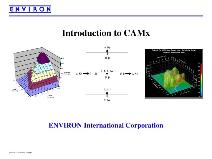
Introduction to CAMx ENVIRON International Corporation
Topics • Conceptual Overview • Ozone Chemistry • Modeling Atmospheric Dispersion • Description of CAMx • Model Design • Comparison to Other Models • Application of CAMx • Model Setup
Conceptual OverviewIntroduction to Atmospheric Dispersion • All models solve some form of the Continuity Equation • Relates changes in pollutant concentration to: • “Dispersion” • Advection (transport by mean/resolved wind) • Turbulent diffusion (transport by unresolved motion) • Chemical reactions • Deposition • Emissions
Conceptual OverviewGeneral Form of the Continuity Equation(Eulerian Form) Mathematical solution (integration) of the general form is difficult • Simplifying assumptions are required
Conceptual OverviewThree General Types of Air Quality Models • Lagrangian types -- Coordinate system follows air parcels • Eulerian types – Coordinate system is fixed in space • Hybrid types – Incorporate features of Lagrangian types into an Eulerian framework
Conceptual OverviewLagrangian Models • Many simplifying assumptions • Air parcel coherency • Break down quickly, especially in complex wind flows • Cost-effective solution at relatively close range for a relatively small number of sources • Readily produce source-receptor relationships • Severe technical limitations for: • Large numbers of sources • Regional-scale transport applications • Non-linearly reactive pollutants
Conceptual OverviewLagrangian Models • Gaussian Plume Models • The earliest air models • Many simplifying assumptions provide closed-form analytical solutions • Steady-state (i.e., time invariant) • Spatially uniform (homogeneous) dispersion • Inert or first-order decay • Examples include: • ISC • COMPLEX • RTDM • AERMOD
Conceptual OverviewLagrangian Models • Gaussian Puff Models • Fewer simplifying assumptions • Retain plume coherency assumption • Employ analytical solutions for each puff, but: • Must track large numbers of puffs • Examples include: • CALPUFF • SCIPUFF • Some models developed for individual reactive plumes; e.g., RPM • Numerical solution methods needed for chemistry • Chemical interactions between puffs, segments, or particles cannot be fully treated
Conceptual OverviewEulerian Models • Generally considered to be technically superior • Allow more comprehensive, explicit treatment of • Physical processes • Chemical processes • Interactions of numerous sources • Require sophisticated solution methods • Employ discrete time steps and operator splitting • Computational grid (“grid models”) • Relatively expensive to apply for long periods
Conceptual OverviewEulerian Models • Subgrid resolution can be a limitation • As grid size and time step are reduced • Accuracy increases, but • Computational time increases • Advanced grid models can • Employ improved accuracy in critical locations • Allow cost effective application on urban to regional scales
Conceptual OverviewEulerian Models • Before source apportionment techniques, many runs were required to: • Establish source-receptor relationships • Evaluate effective control strategies • Examples of early photochemical grid models include: • UAM-IV • RADM • CALGRID
Conceptual OverviewHybrid Models • Incorporate features of Lagrangian models into grid model framework • Overcome many of the limitations of sub-grid processes • Provides practical advantages of Lagrangian models, by development of: • Plume-in-Grid (PiG) sub-models • Variable (nested) grid resolution • Source apportionment techniques • Capitalize on availability of low-cost high-speed computers
Conceptual OverviewHybrid Models • Examples of hybrid photochemical grid models include: • CAMx • MODELS3/CMAQ • UAM-V
Conceptual OverviewSummary • Photochemical hybrid models • Preferred means for addressing complex and nonlinear processes affecting reactive tropospheric air pollutants • Variable grid spacing (nested grids) • Lagrangian PiG sub-models to treat subgrid plume dispersion and chemistry • Source apportionment and process analysis tools • These models invoke fewer assumptions, but require: • More computer resources • Sophisticated numerical integration methods
Description of CAMxComprehensive Air quality Model with extensions (CAMx), Version 4.00 • 3-D Eulerian/hybrid tropospheric photochemical transport model • Treats emissions, chemistry, dispersion, removal • Chemical species • Photochemical gasses (NOx, VOC, CO, O3) • Aerosols (sulfate, nitrate, organics, inert) • Applicable scales • From individual point sources (< 1 km) • To regional (>1000 km)
Description of CAMx CAMx v4.00 • Unifies features required of “state-of-the-science” models • New coding of several industry-accepted algorithms • Computational and memory efficient • Easy to use • Modular framework permits easy substitution of revised and/or alternate algorithms • Publicly available (www.camx.com)
Description of CAMx CAMx v4.00 • Technical features: • Grid nesting • Horizontal and vertical nesting • Supports multiple levels • Variable meshing factors • Plume-in-Grid (PiG) sub-model • Multiple, fast and accurate chemical mechanisms • Mass conservative and mass consistent transport scheme
Description of CAMx CAMx v4.00 • Multiple map projections • Geodetic (latitude/longitude) • Universal Transverse Mercator (UTM) • Lambert Conformal Projection (LCP) • Rotated Polar Stereographic Projection (PSP) • Multiple probing tools • Ozone Source Apportionment Technology (OSAT) • Decoupled Direct Method (DDM) of sensitivity analysis • Process Analysis tools (IPR, IRR, CPA)
Description of CAMxTechnical Approach • Overview • Solves continuity equation for each species • Time splitting operation • Each process solved individually each time step, each grid • Master time step: • Maintains stable solution of transport on master grid • Multiple nested grid steps per master step • Multiple chemistry steps per master step
Description of CAMxTechnical Approach • Transport • Advection and diffusion solvers are mass conservative • 3-D advection is mass consistent • Linked via divergent atmospheric incompressible continuity equation • Order of east-west and north-south advection alternates each master step • Two options for horizontal advection solver: • Bott (1989): area-preserving flux-form solver • Colella and Woodward (1984): piecewise-parabolic method
Description of CAMxTechnical Approach • Vertical transport solved with implicit scheme • Resolved vertical velocity • Mass exchange across variable vertical layer structure • Vertical diffusion solved with implicit scheme • Dry deposition rates used as surface boundary condition • Horizontal diffusion solved with explicit scheme • 2-D simultaneous
Description of CAMxTechnical Approach • Pollutant removal • Dry deposition • First order removal rate based on deposition velocity (Weseley, 1989) • Dependent upon: season, land cover, solar flux, surface stability, surface wetness, gas solubility and diffusivity, aerosol size • Wet scavenging • First order removal rate based on scavenging coefficient • Gas rates depend upon solubility and diffusivity • Aerosol rates depend upon size • Separate in-cloud and below-cloud rates (Seinfeld and Pandis, 1998)
Description of CAMxTechnical Approach • Photochemistry • CBM-IV (Gery et al., 1989) • 3 variations available • SAPRC99 (Carter, 2000) • Chemically up-to-date • Tested extensively against environmental chamber data • Uses a different approach for VOC lumping • All mechanisms are balanced for nitrogen conservation • Photolysis rates derived from TUV preprocessor • Can be affected by cloud optical depth
Description of CAMxTechnical Approach • Gas-phase chemistry solvers • Most “expensive” component of simulation • CAMx CMC solver • Increases efficiency and flexibility • Adaptive hybrid approach: • Radicals (fastest reactions) – in steady state • Fast state species – second-order Runge-Kutta • Slow state species – solved explicitly • “Adaptive” = number of fast species can change according to chemical regime
Description of CAMxTechnical Approach • Implicit-Explicit Hybrid solver (Sun et al, 1994) • Accuracy comparable to reference methods (LSODE) • IEH vs. CMC: • Accuracy similar during the day • IEH more accurate during the night • IEH several times slower
Description of CAMxTechnical Approach • Aerosol chemistry • Gas-phase mechanism (CBM-IV Mech 3) with: • Additional biogenic olefin (terpenes) • Condensible organic gas species • Chlorine and HCl chemistry • Homogeneous SO2 to sulfate • Photochemical production of nitric acid • Aerosol mechanism calculates: • Aqueous SO2 to sulfate (CMAQ/RADM-AQ) • Condensible organic gasses to organic aerosols (SOAP) • NO3/SO4/NH3/Na/Cl equilibrium (ISORROPIA) • Size spectrum is static, user-defined
Description of CAMxTechnical Approach • Aerosol species treated: • Sulfate • Nitrate • Ammonium • Sodium • Chloride • Secondary Organics • Primary Organics • Elemental Carbon • Primary Fine (+dust) • Primary Coarse (+dust)
Description of CAMxTechnical Approach • Plume-in-Grid (PiG) • Resolves chemistry/dispersion of large NOx plumes • Tracks plume segments (puffs) in Lagrangian frame • Each puff moved independently by local winds • Puff growth (diffusion) determined by local diffusion coefficients • GREASD PiG: fast, conceptually simple • Reduced NOx chemistry set (NO-NO, NOx/ozone equilibrium, HNO3 production) • Puffs leak mass according to growth rates and grid cell size • Puffs terminated by age or sufficiently dilute NOx
Description of CAMxTechnical Approach • Probing Tools • Utilize CAMx routines for all dispersion and chemistry • Ozone Source Apportionment Technology (OSAT) • Determines source area/category contribution to ozone anywhere in the domain • Uses tracers to track NOx and VOC precursor emissions, ozone production/destruction, and initial/boundary conditions • Estimates ozone production as NOx- or VOC formed
Description of CAMxTechnical Approach • HOWEVER: cannot quantify ozone response to NOx or VOC controls • Chemical allocation methodologies: • OSAT: standard approach • APCA: attributes ozone production to anthropogenic (controllable) sources only • GOAT: tracks ozone based on where it formed, not where precursors were emitted
Description of CAMxTechnical Approach • Decoupled Direct Method (DDM) for sensitivity analysis • Calculates pollutant concentration sensitivity to input parameters • First-order sensitivity to emissions, initial/boundary conditions • Allows estimates of effects of emission changes • Allows ranking of source region/categories by their importance to ozone formation • Slower than OSAT, but: • Provides information for all species (not just ozone) • More flexible in selecting which parameters to track
Description of CAMxTechnical Approach • Process Analysis (PA) • Designed to provide in-depth analyses of all physical and chemical processes operating in model • Operates on user-defined species and any portion of the modeling grid • Three components: • Integrated Process Rate (IPR): provides detailed process rate information for each physical process (emissions, advection, diffusion, chemistry, deposition) • Integrated Reaction Rate (IRR): provides detailed reaction rate information for all chemical reactions • Chemical Process Analysis (CPA): like IRR, but designed to be more user-friendly and accessible
Description of CAMxInput Requirements • Meteorology (Fortran binary) • 3-D time-varying fields to define the state of the troposphere • Winds, temperature, pressure, humidity, clouds, rain, turbulent diffusion rates • Affects transport, chemistry, deposition • Defines vertical grid structure • Air quality (UAM Fortran binary) • Initial and boundary conditions • Time constant or varying • All species or a sub-set
Description of CAMxInput Requirements • Emissions (UAM Fortran binary) • 2-D time varying emission fields • Individual time-varying elevated point sources • Other Inputs • User control file (text) • Chemistry parameters file (text) • Land use / land cover (Fortran binary) • Albedo / haze / ozone column definition (text) • Photolysis rates lookup table (text) • Probing Tool definition files (text)
Description of CAMxModel Output • Average concentration (UAM Fortran binary) • 2-D (surface) or 3-D time varying • User-selected species (ppm gasses, g/m3 aerosols) • Separate master grid and fine grid files • Instant concentration (UAM Fortran binary) • 3-D time varying (output last 2 hours of simulation for model restart) • All species (mol/m3 gasses, g/m3 aerosols) • Separate master grid and fine grid files
Description of CAMxModel Output • Deposition (UAM Fortran binary) • 2-D time varying • User-selected species • Dry deposition velocity (m/s) • Dry and wet deposition fluxes (mol/ha gasses, g/ha aerosols) • Precipitation liquid concentration (mol/l gasses, g/l aerosols) • Separate master grid and find grid files
Description of CAMxModel Output • PiG restart (Fortran binary) • All relevant PiG information for model restart • Diagnostic files (text) • Repeat run control parameters and I/O file names • Diagnostic messages and warning/error messages • CPU timing • Mass budgets
Description of CAMxModel Output • Probing Tool files • Master and fine grid instantaneous tracer files (UAM Fortran binary) • Master and fine grid average tracer and PA rates files (UAM Fortran binary) • OSAT and DDM receptor file (text) • Tracer/sensitivity concentrations at discrete receptors • IPR and IRR rates files (Fortran binary) • Time-varying rate information for user-selected cells
Description of CAMxComputer Requirements • Dependent upon size of CAMx application • Standard model vs. large Probing Tool configuration • Number of nested grids needed and number of cells per grid • Chemistry mechanism • SAPRC99 slower than CBM-IV • PM chemistry slows model significantly • Chemistry solver • IEH slower than CMC • Plan according to episode length and desired throughput for desired number of simulations
Description of CAMxComputer Requirements Example: CAMx application on 1 Ghz Pentium III PC CBM-IV Mech 3 (no aerosols), CMC solver
Description of CAMxComputer Requirements • Recommended hardware – Linux workstation • Minimum 256 Mb memory • Fastest affordable PC chipset available • Minimum 10 Gb available disk space • Graphics monitor and associated drivers • Recommended software • Portland Group F77/F90 compiler for Linux • PAVE, Vis5d, Surfer (or some other graphics viewer) • Ancillary support software for pre- and post-processing • SAS (for EMS-95), ArcInfo or other GIS systems • MM5, RAMS, NCAR Graphics (for meteorological preprocessing)
Application of CAMxCAMx Setup -- Air Quality Definition • Initial Conditions • Model starts from this definition • May be defined by ambient measurements • Usually available data is sparse, not 3-D • May be defined as spatially invariant • Need to spin up model over a day or more to remove • Boundary Conditions • Lateral boundaries (may be time, space varying) • Concentrations aloft (space invariant)
Application of CAMxCAMx Setup – Chemistry Definition • Chemical Processes in CAMx • Gas phase chemistry • Define mechanism, rate constants, photolysis rates • Aerosol chemistry • Define species, representative sizes, density • Dry deposition • Define Henry’s law solubility, diffusivity, reactivity • Wet deposition • Define Henry’s law solubility
Application of CAMxCAMx Setup – Chemistry Definition • Contents of chemistry parameters file • Mechanism (choose from 1 through 5 or inert) • Photolysis reaction parameters and options • Gas phase species list • Lower bound values • Deposition parameters (KH, diffusivity, reactivity) • Aerosol species list (mechanism 4 only) • Lower bound values • Size parameters • Density • Gas phase reaction rate constants
Application of CAMxCAMx Setup – Chemistry Definition Mechanism options in v4.00
Application of CAMxCAMx Setup -- Chemistry Definition • Photolysis Rates Input • Two options: • Directly input using a lookup table, or • Set by ratio to a reaction given in lookup table • Thus, must directly input at least one reaction • Input files: • Chemistry parameters • Specifies photolysis rate options by reaction number
Application of CAMxCAMx Setup – Chemistry Definition • Photolysis Rate Input File • Look-up tables for all directly specified photolysis reactions • Function of: • Zenith angle • Altitude • UV Albedo • Haze opacity • Ozone column • Prepared using TUV light model from NCAR