Download
1 / 21
210 likes | 315 Vues
Stochastic Optimization for Markov Modulated Networks with Application to Delay Constrained Wireless Scheduling. A 1 (t). State 1. State 3. A 2 (t). State 2. Control-Dependent Transition Probabilities. A L (t ). Michael J. Neely University of Southern California

E N D
Stochastic Optimization for Markov Modulated Networks with Application to Delay Constrained Wireless Scheduling A1(t) State 1 State 3 A2(t) State 2 Control-Dependent Transition Probabilities AL(t) Michael J. Neely University of Southern California http://www-rcf.usc.edu/~mjneely Proc. 48th IEEE Conf. on Decision and Control (CDC), Dec. 2009 *Sponsored in part by the DARPA IT-MANET Program, NSF OCE-0520324, NSF Career CCF-0747525
Motivating Problem: • Delay Constrained Opportunistic Scheduling • Status Quo: • Lyapunov Based Max-Weight: [Georgiadis, Neely, Tassiulas F&T 2006] • Treats stability/energy/thruput-utility with low complexity • Cannot treat average delay constraints • Dynamic Programming / Markov Decision (MDP) Theory: • Curse of Dimensionality • Need to know Traffic/Channel Probabilities A1(t) S1(t) A2(t) S2(t) AK(t) SK(t)
Insights for Our New Approach: • Combine Lyapunov/Max-Weight Theory with Renewals/MDP A1(t) S1(t) • Lyapunov Functions • Max-Weight Theory • Virtual Queues • Renewal Theory • Stochastic Shortest Paths • MDP Theory A2(t) S2(t) • Consider “Small” number of Control-Driven Markov States • K Queues with Avg. Delay Constraints (K “small”) • N Queues with Stability Constraints (N arbitrarily large) AK(t) SK(t) AK+1(t) SK+1(t) Example: AM(t) SM(t) Delay Constrained Not Delay Constrained
Key Results: • Unify Lyapunov/Max-Weight Theory with Renewals/MDP “Weighted Stochastic Shortest Path (WSSP)” “Max Weight (MW)” • Treat General Markov Decision Networks • Use Lyapunov Analysis and Virtual Queues to Optimize • and Compute Performance Bounds • Use Existing SSP Approx Algs (Robbins-Monro) to Implement • For Example Delay Problem: • Meet all K Average Delay Constraints, Stabilize all N other queues • Utility close to optimal, with tradeoff in delay of N other queues • All Delays and Convergence Times are polynomialin (N+K) • Per-Slot Complexity geometric in K
General Problem Formulation: (slotted time t = {0,1,2,…}) • Qn(t) = Collection of N queues to be stabilized • S(t) = Random Event (e.g. random traffic, channels) • Z(t) = Markov State Variable (|Z| states) • I(t) = Control Action (e.g. service, resource alloc.) • xm(t) = Additional Penalties Incurred by action on slot t Qn(t) mn(t) Rn(t) Control-Dependent Transition Probs: General functions for m(t), R(t), x(t): mn(t) = mn(I(t), S(t), Z(t)) Rn(t) = Rn(I(t), S(t), Z(t)) xm(t) = xm(I(t), S(t), Z(t)) State 1 State 3 I(t), S(t) Z(t) Z(t+1) State 2
General Problem Formulation: (slotted time t = {0,1,2,…}) • Qn(t) = Collection of N queues to be stabilized • S(t) = Random Event (e.g. random traffic, channels) • Z(t) = Markov State Variable (|Z| states) • I(t) = Control Action (e.g. service, resource alloc.) • xm(t) = Additional Penalties Incurred by action on slot t Qn(t) mn(t) Rn(t) General functions for m(t), R(t), x(t): Goal: Minimize: x0 Subject to:xm< xmav, all m Qm stable , all m mn(t) = mn(I(t), S(t), Z(t)) Rn(t) = Rn(I(t), S(t), Z(t)) xm(t) = xm(I(t), S(t), Z(t))
Applications of this Formulation: • For K of the queues, let: Z(t) = (Q1(t), …, QK(t)) • These K have Finite Buffer: Qk(t) in {0, 1, …, Bmax} • Cardinality of states: |Z| = (Bmax +1)K • Recall: Penalties have the form: xm(t) = xm(I(t), S(t), Z(t)) • Penalty for Congestion: • Define Penalty: xk(t) = Zk(t) • Can then do one of the following (for example): • Minimize: xk • Minimize: x1+ … + xK • Constraints:xk < xkav
Applications of this Formulation: • For K of the queues, let: Z(t) = (Q1(t), …, QK(t)) • These K have Finite Buffer: Qk(t) in {0, 1, …, Bmax} • Cardinality of states: |Z| = (Bmax +1)K • Recall: Penalties have the form: xm(t) = xm(I(t), S(t), Z(t)) • 2) Penalty for Packet Drops: • Define Penalty: xk(t) = Dropsk(t) • Can then do one of the following (for example): • Minimize: xk • Minimize: x1+ … + xK • Constraints:xk < xkav
Applications of this Formulation: • For K of the queues, let: Z(t) = (Q1(t), …, QK(t)) • These K have Finite Buffer: Qk(t) in {0, 1, …, Bmax} • Cardinality of states: |Z| = (Bmax +1)K • Recall: Penalties have the form: xm(t) = xm(I(t), S(t), Z(t)) • A Nice Trick for Average Delay Constraints: • Suppose we want: W < 5 slots : • Define Penalty: xk(t) = Qk(t) – 5 xArrivalsk(t) • Then by Little’s Theorem… • xk < 0 equivalent to: Qk – 5 xlk < 0 • equivalent to: Wkxlk – 5 xlk < 0 • equivalent to: Wk < 5
Solution to the General Problem: Minimize: x0 Subject to:xm< xmav, all m Qk stable , all k • Define Virtual Queues for Each Penalty Constraint: • Define Lyapunov Function: • L(t) = Qk(t)2 + Ym(t)2 Ym(t) xmav xm(t)
Solution to the General Problem: • Define Forced Renewals every slot i.i.d. probability d>0 State 1 State 3 Renewal State 0 State 2 Example for K Delay-Constrained Queue Problem: Every slot, with probability d, drop all packets in all K Delay-Constrained Queues (loss rate < Bmaxd) Renewals “Reset” the system
Solution to the General Problem: • Define Variable Slot Lyapunov Drift over Renewal Period DT(Q(t), Y(t)) = E{L(t+T) – L(t)| Q(t), Y(t)} where T = Random Renewal Period Duration t t+T • Control Rule: Every Renewal time t, observe queues, • Take action to Min the following over 1 Renewal Period: • Minimize: DT(Q(t), Y(t)) + VE{ x0(t) | Q(t), Y(t)} t+T-1 t=t *Generalizes our previous max-weight rule from [F&T 2006] !
Minimize: DT(Q(t), Y(t)) + VE{ x0(t) | Q(t), Y(t)} Max-Weight (MW) Weighted Stochastic Shortest Path (WSSP) • Suppose we implement a (C,e)-approximate SSP, so that • every renewal period we have… • Achieved Cost < Optimal SSP + C + e[ Qk+Ym+ V] Can achieve this using approximate DP Theory, Neurodynamic Programming, etc., (see [Bertsekas, TsitsiklisNeurodynamic Programming]) together with a Delayed-Queue-Analysis. t+T-1 t=t
Theorem: If there exists a policy that meets all Constraints with “emax slackness,” then any (C, e) approximate SSP implementation yields: All (virtual and actual) Queues Stable, and: E{Qsum} < (B/d + Cd) + V(ed + xmax) emax - ed All Time Average Constraints are satisfied ( xm < xmav) Time Average Cost satisfies: x0 < x0(optimal) + (B/d + Cd) + ed(1 + xmax/emax) V (recall that d = forced renewal probability)
Proof Sketch: (Consider exact SSP for simplicity) DT(Q(t), Y(t)) + VE{ x0(t) | Q(t), Y(t)} < B + VE{ x0(t) | Q(t), Y(t)} -Qk(t)E{ [mk(t) – Rk(t)] | Q(t), Y(t)} -Ym(t)E{ [xmav – xm(t)] | Q(t), Y(t)} t+T-1 t+T-1 t+T-1 t+T-1 [We take control action to minimize the Right Hand Side above over the Renewal Period. This is the Weighted SSP problem of interest] t=t t=t t=t t=t
Proof Sketch: (Consider exact SSP for simplicity) DT(Q(t), Y(t)) + VE{ x0(t) | Q(t), Y(t)} < B + VE{ x0*(t) | Q(t), Y(t)} -Qk(t)E{ [mk*(t) – Rk*(t)] | Q(t), Y(t)} -Ym(t)E{ [xmav – xm*(t)] | Q(t), Y(t)} t+T-1 t+T-1 t+T-1 t+T-1 [We can thus plug in any alternative control policy in the Right Hand Side, including the one that yields the optimum time average subject to all time average constraints] t=t t=t t=t t=t
Proof Sketch: (Consider exact SSP for simplicity) DT(Q(t), Y(t)) + VE{ x0(t) | Q(t), Y(t)} < B + VE{ x0*(t) | Q(t), Y(t)} -Qk(t)E{ [mk*(t) – Rk*(t)] | Q(t), Y(t)} -Ym(t)E{ [xmav – xm*(t)] | Q(t), Y(t)} t+T-1 t+T-1 t+T-1 t+T-1 [Note by RENEWAL THEORY, the infinite horizon time average is exactly achieved over any renewal period ] t=t t=t t=t t=t
Proof Sketch: (Consider exact SSP for simplicity) DT(Q(t), Y(t)) + VE{ x0(t) | Q(t), Y(t)} X0(optimum)E{T} < B + VE{ x0*(t) | Q(t), Y(t)} 0 -Qk(t)E{ [mk*(t) – Rk*(t)] | Q(t), Y(t)} 0 -Ym(t)E{ [xmav – xm*(t)] | Q(t), Y(t)} t+T-1 t+T-1 t+T-1 t+T-1 [Note by RENEWAL THEORY, the infinite horizon time average is exactly achieved over any renewal period ] t=t t=t t=t t=t
Proof Sketch: (Consider exact SSP for simplicity) DT(Q(t), Y(t)) + VE{ x0(t) | Q(t), Y(t)} < B + VX0(optimum)E{T} t+T-1 [Sum the resulting telescoping series to get the utility performance bound! ] t=t
Implementation of Approximate Weighted SSP: • Use a simple 1-step Robbins-Monro Iteration • with past history Of W samples {S(t1), S(t2), …, S(tW)}. • To avoid subtle correlations between samples and • queue weights, use a Delayed Queue Analysis. • Algorithm requires no a-priori knowledge of statistics, • and takes roughly |Z| operations per slot to perform • Robbins-Monro. Convergence and Delay are log(|Z|). • For K Delay constrained queues, |Z| = BmaxK • (geometric in K). Can modify implementation for • constant per-slot complexity, but then convergence time • is geometric in K. (Either way, we want K small).
Conclusions: • Treat general Markov Decision Networks • Generalize Max-Weight/Lyapunov Optimization to • Min Weighted Stochastic Shortest Path (W-SSP) • Can solve delay constrained network problems: • Convergence Times, Delays Polynomial in (N+K) • Per-Slot Computation Complexity of Solving • Robbins-Monro is geometric in K. (want K small) A1(t) A2(t) AL(t) State 1 State 3 State 2 Control-Dependent Transition Probabilities