Hidden Markov Models

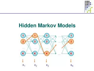
1. 1 2 2 1 1 1 1 … 2 2 2 2 … K … … … … x1 K K K K x2 x3 xK … Hidden Markov Models

2. Viterbi, Forward, Backward VITERBI Initialization: V0(0) = 1 Vk(0) = 0, for all k > 0 Iteration: Vl(i) = el(xi) maxkVk(i-1) akl Termination: P(x, *) = maxkVk(N) • FORWARD • Initialization: • f0(0) = 1 • fk(0) = 0, for all k > 0 • Iteration: • fl(i) = el(xi) k fk(i-1) akl • Termination: • P(x) = k fk(N) BACKWARD Initialization: bk(N) = 1, for all k Iteration: bl(i) = k el(xi+1) akl bk(i+1) Termination: P(x) = k a0k ek(x1) bk(1)

3. Posterior Decoding P(i = k | x) = P(i = k , x)/P(x) = P(x1, …, xi, i = k, xi+1, … xn) / P(x) = P(x1, …, xi, i = k) P(xi+1, … xn | i = k) / P(x) = fk(i) bk(i) / P(x) We can now calculate fk(i) bk(i) P(i = k | x) = ––––––– P(x) Then, we can ask What is the most likely state at position i of sequence x: Define ^ by Posterior Decoding: ^i = argmaxkP(i = k | x)

4. Posterior Decoding • For each state, • Posterior Decoding gives us a curve of likelihood of state for each position • That is sometimes more informative than Viterbi path * • Posterior Decoding may give an invalid sequence of states (of prob 0) • Why?

5. Posterior Decoding x1 x2 x3 …………………………………………… xN • P(i = k | x) = P( | x) 1(i = k) =  {:[i] = k}P( | x) State 1 P(i=l|x) l k 1() = 1, if  is true 0, otherwise

6. Variants of HMMs

7. Higher-order HMMs • How do we model “memory” larger than one time point? • P(i+1 = l | i = k) akl • P(i+1 = l | i = k, i -1 = j) ajkl • … • A second order HMM with K states is equivalent to a first order HMM with K2 states aHHT state HH state HT aHT(prev = H) aHT(prev = T) aHTH state H state T aHTT aTHH aTHT state TH state TT aTH(prev = H) aTH(prev = T) aTTH

8. Similar Algorithms to 1st Order • P(i+1 = l | i = k, i -1 = j) • Vlk(i) = maxj{ Vkj(i – 1) + … } • Time? Space?

9. Modeling the Duration of States 1-p Length distribution of region X: E[lX] = 1/(1-p) • Geometric distribution, with mean 1/(1-p) This is a significant disadvantage of HMMs Several solutions exist for modeling different length distributions X Y p q 1-q

10. Example: exon lengths in genes

11. Solution 1: Chain several states p 1-p X Y X X q 1-q Disadvantage: Still very inflexible lX = C + geometric with mean 1/(1-p)

12. Solution 2: Negative binomial distribution Duration in X: m turns, where • During first m – 1 turns, exactly n – 1 arrows to next state are followed • During mth turn, an arrow to next state is followed m – 1 m – 1 P(lX = m) = n – 1 (1 – p)n-1+1p(m-1)-(n-1) = n – 1 (1 – p)npm-n p p p 1 – p 1 – p 1 – p Y X(n) X(1) X(2) ……

13. Example: genes in prokaryotes • EasyGene: Prokaryotic gene-finder Larsen TS, Krogh A • Negative binomial with n = 3

14. Solution 3: Duration modeling Upon entering a state: • Choose duration d, according to probability distribution • Generate d letters according to emission probs • Take a transition to next state according to transition probs Disadvantage: Increase in complexity of Viterbi: Time: O(D) Space: O(1) where D = maximum duration of state F d<Df xi…xi+d-1 Pf Warning, Rabiner’s tutorial claims O(D2) & O(D) increases

15. Viterbi with duration modeling emissions emissions Recall original iteration: Vl(i) = maxk Vk(i – 1) akl el(xi) New iteration: Vl(i) = maxk maxd=1…DlVk(i – d) Pl(d) akl j=i-d+1…iel(xj) F L d<Df d<Dl Pl Pf transitions xi…xi + d – 1 xj…xj + d – 1 Precompute cumulative values

16. Proteins, Pair HMMs, and Alignment

17. A state model for alignment M (+1,+1) Alignments correspond 1-to-1 with sequences of states M, I, J I (+1, 0) J (0, +1) -AGGCTATCACCTGACCTCCAGGCCGA--TGCCC--- TAG-CTATCAC--GACCGC-GGTCGATTTGCCCGACC IMMJMMMMMMMJJMMMMMMJMMMMMMMIIMMMMMIII

18. Let’s score the transitions s(xi, yj) M (+1,+1) Alignments correspond 1-to-1 with sequences of states M, I, J s(xi, yj) s(xi, yj) -d -d I (+1, 0) J (0, +1) -e -e -AGGCTATCACCTGACCTCCAGGCCGA--TGCCC--- TAG-CTATCAC--GACCGC-GGTCGATTTGCCCGACC IMMJMMMMMMMJJMMMMMMJMMMMMMMIIMMMMMIII

19. Alignment with affine gaps – state version Dynamic Programming: M(i, j): Optimal alignment of x1…xi to y1…yjending in M I(i, j): Optimal alignment of x1…xi to y1…yj ending in I J(i, j): Optimal alignment of x1…xi to y1…yjending in J The score is additive, therefore we can apply DP recurrence formulas

20. Alignment with affine gaps – state version Initialization: M(0,0) = 0; M(i, 0) = M(0, j) = -, for i, j > 0 I(i,0) = d + ie; J(0, j) = d + je Iteration: M(i – 1, j – 1) M(i, j) = s(xi, yj) + max I(i – 1, j – 1) J(i – 1, j – 1) e + I(i – 1, j) I(i, j) = max d + M(i – 1, j) e + J(i, j – 1) J(i, j) = max d + M(i, j – 1) Termination: Optimal alignment given by max { M(m, n), I(m, n), J(m, n) }

21. Brief introduction to the evolution of proteins Protein sequence and structure Protein classification Phylogeny trees Substitution matrices

22. Structure Determines Function The Protein Folding Problem • What determines structure? • Energy • Kinematics • How can we determine structure? • Experimental methods • Computational predictions

23. Primary Structure: Sequence • The primary structure of a protein is the amino acid sequence

24. Primary Structure: Sequence • Twenty different amino acids have distinct shapes and properties

25. Primary Structure: Sequence A useful mnemonic for the hydrophobic amino acids is "FAMILY VW"

26. Secondary Structure: , , & loops •  helices and  sheets are stabilized by hydrogen bonds between backbone oxygen and hydrogen atoms

27. Tertiary Structure: A Protein Fold

28. Actin structure

29. Actin sequence • Actin is ancient and abundant • Most abundant protein in cells • 1-2 actin genes in bacteria, yeasts, amoebas • Humans: 6 actin genes • -actin in muscles; -actin, -actin in non-muscle cells • ~4 amino acids different between each version MUSCLE ACTIN Amino Acid Sequence 1 EEEQTALVCD NGSGLVKAGF AGDDAPRAVF PSIVRPRHQG VMVGMGQKDS YVGDEAQSKR 61 GILTLKYPIE HGIITNWDDM EKIWHHTFYN ELRVAPEEHP VLLTEAPLNP KANREKMTQI 121 MFETFNVPAM YVAIQAVLSL YASGRTTGIV LDSGDGVSHN VPIYEGYALP HAIMRLDLAG 181 RDLTDYLMKI LTERGYSFVT TAEREIVRDI KEKLCYVALD FEQEMATAAS SSSLEKSYEL 241 PDGQVITIGN ERFRGPETMF QPSFIGMESS GVHETTYNSI MKCDIDIRKD LYANNVLSGG 301 TTMYPGIADR MQKEITALAP STMKIKIIAP PERKYSVWIG GSILASLSTF QQMWITKQEY 361 DESGPSIVHR KCF

30. A related protein in bacteria

31. Relation between sequence and structure

32. Protein Phylogenies • Proteins evolve by both duplication and species divergence

33. Protein Phylogenies – Example

34. PDB Growth New PDB structures

35. Only a few folds are found in nature

36. Substitutions of Amino Acids Mutation rates between amino acids have dramatic differences!

37. Substitution Matrices BLOSUM matrices: • Start from BLOCKS database (curated, gap-free alignments) • Cluster sequences according to > X% identity • Calculate Aab: # of aligned a-b in distinct clusters, correcting by 1/mn, where m, n are the two cluster sizes • Estimate P(a) = (bAab)/(c≤dAcd); P(a, b) = Aab/(c≤dAcd)

38. Probabilistic interpretation of an alignment An alignment is a hypothesis that the two sequences are related by evolution Goal: Produce the most likely alignment Assert the likelihood that the sequences are indeed related

39. A Pair HMM for alignments Model M 1 – 2 This model generates two sequences simultaneously Match/Mismatch state M: P(x, y) reflects substitution frequencies between pairs of amino acids Insertion states I, J: P(x), P(y) reflect frequencies of each amino acid : set so that 1/2 is avg. length before next gap :set so that 1/(1 – ) is avg. length of a gap M P(xi, yj) 1 –  1 –      I P(xi) J P(yj) optional

40. A Pair HMM for unaligned sequences Model R Two sequences are independently generated from one another P(x, y | R) = P(x1)…P(xm) P(y1)…P(yn) = i P(xi) j P(yj) 1 1 J P(yj) I P(xi)

41. To compare ALIGNMENT vs. RANDOM hypothesis 1 – 2 Every pair of letters contributes: M • (1 – 2) P(xi, yj) when matched •  P(xi) P(yj) when gapped R • P(xi) P(yj) in random model Focus on comparison of P(xi, yj) vs. P(xi) P(yj) M P(xi, yj) 1 –  1 –      I P(xi) J P(yj) 1 1 J P(yj) I P(xi)

42. To compare ALIGNMENT vs. RANDOM hypothesis 1 – 2 Every pair of letters contributes: M • (1 – 2) P(xi, yj) when matched •  P(xi) P(yj) when gapped • Some extra term for gap opening R • P(xi) P(yj) in random model Focus on comparison of P(xi, yj) vs. P(xi) P(yj) M P(xi, yj) 1 – 2 1 – 2 (1 – ) –––––––– (1 – 2)   I P(xi) J P(yj) Equivalent! 1 1 J P(yj) I P(xi)

43. To compare ALIGNMENT vs. RANDOM hypothesis Idea: We will divide M alignment score by R score, and take logarithms Let P(xi, yj) s(xi, yj) = log ––––––––– + log (1 – 2) P(xi) P(yj)  (1 – ) P(xi) d = – log ––––––––––––– (1 – 2) P(xi)  P(xi) e = – log –––––– P(xi) =Defn substitution score =Defn gap initiation penalty =Defn gap extension penalty

44. The meaning of alignment scores • The Viterbi algorithm for Pair HMMs corresponds exactly to global alignment DP with affine gaps VM(i, j) = max { VM(i – 1, j – 1), VI( i – 1, j – 1) – d, Vj( i – 1, j – 1) } + s(xi, yj) VI(i, j) = max { VM(i – 1, j) – d, VI( i – 1, j) – e } VJ(i, j) = max { VM(i – 1, j) – d, VI( i – 1, j) – e } • s(.,.) (1 – 2) ~how often a pair of letters substitute one another •  1/mean length of next gap • (1 – ) / (1 – 2) 1/mean arrival time of next gap

45. The meaning of alignment scores Match/mismatch scores: P(xi, yj) s(a, b)  log –––––––––– (ignore log(1 – 2) for the moment) P(xi) P(yj) Example: Genes between human and mouse genes have average conservation of 80% • Let’s calculate this way the substitution score for a match: P(a, a) + P(c, c) + P(g, g) + P(t, t) = 0.8  P(x, x) = 0.2 P(a) = P(c) = P(g) = P(t) = 0.25 s(x, x) = log [ 0.2 / 0.252 ] = 1.163 • …and for a mismatch: P(a, c) +…+P(t, g) = 0.2  P(x, yx) = 0.2/12 = 0.0167 s(x, y  x) = log[ 0.0167 / 0.252 ] = -1.322 • What ratio matches/(matches + mism.) gives score 0? x(#match) – y(#mism) = 0 1.163 (#match) – 1.322 (#mism) = 0 #match = 1.137(#mism) matches = 53.2%