Download
1 / 26
280 likes | 499 Vues
Fluid Dynamics – Gollub – Lecture #2. Outline – Lecture #2 Reynolds number and other dimensionless parameters Hydrodynamic similarity Important steady flows: shear flow; tubes Low Re flows: Stokes flow Flow around particles Drag on particles at low Re Drag at higher Re

E N D
Fluid Dynamics – Gollub – Lecture #2 • Outline – Lecture #2 • Reynolds number and other dimensionless parameters • Hydrodynamic similarity • Important steady flows: shear flow; tubes • Low Re flows: Stokes flow • Flow around particles • Drag on particles at low Re • Drag at higher Re • Sedimentation; particle interactions • Lubrication forces • Boundary layers • Vorticity and vortices • Surface waves
Boundary conditions • Generally, both normal and tangential components of velocity are zero at a solid surface. • No-slip usually works well down to a few nm scales, except in special cases (hydrophobic boundaries in microfluidics; dilute gasses). • Pressure is usually continuous across fluid boundaries (except for surface tension effects). • What would happen at a gas/liquid boundary? (Movie: gas_fluid)
Reynolds number (and other dimensionless parameters) • Ratio of advective (or inertial) to viscous terms in N-S: • Re for stirring coffee ~1000; for a bacterium in water, Re~ 10-5. • Many other dimensionless parameters arise; e.g. • Peclet number compares advection and convection terms.
Hydrodynamic similarity • If velocities, lengths, and pressures are made dimensionless using U,L, U2 , Then the steady N-S equation looks like this: The only parameter is Re. So steady flows at the same Re driven by geometrically similar boundaries will be identical when expressed non-dimensionally.
Simple shear flow • For a simple parallel shear flow (no gravity; no horizontal pressure gradient), N-S reduces to • Gives linear profile for a moving wall near a static one. • Wall shear stress in a fluid is very different from solid friction. • Even better to use ball bearings so that there is no relative velocity.
Other steady flows: tubes and surfaces • Flow in a tube with pressure gradient G: Solve N-S in cylindrical coordinates for the speed and flux. • Entrance length: Momentum diffuses gradually; profile evolves. • Flow on an inclined surface at angle . Parabolic, but no gradient at the surface.
More on flow in tubes • The drag on a tube in the laminar regime can be found by taking the gradient of the velocity at the wall and multiplying by the area of the wall, to obtain D=8UL. • If Re is defined as Re=(2a)U/, then it is found that turbulence occurs around 2000-4000, but it can be much higher if perturbations are avoided. • In the turbulent regime, which does arise in arterial flow, the drag is augmented by a further factor f(Re) that grows slowly with Re, e.g. 7 at 10,000 and 20 at 100,000.
Stokes Flow- Low Re • Start from Navier-Stokes: • Look at steady solutions at low Re (“creeping flow”): • Movie of reversible stokes flow by G.I.Taylor
Flow around a spherical particle • Pressure satisfies Laplace’s equation. Solve in spherical coordinates with =0 in the flow direction. Sketch it. • Note slow falloff; influence over large distances. • Pressure is asymmetric. • Use the rate of strain tensor to find the stress, which turns out to be uniform over the particle’s surface. Multiplying by the area gives the famous Stokes drag. It turns out that 2/3 of this is skin friction (viscosity) and 1/3 is due to the pressure force on the shape (non-dissip.)
Drag - continued • Q: Can we apply the drag just computed for a particle at rest to a moving particle in a quiescent fluid? If so why? • The terminal velocity under a constant gravity or electric field varies as a2, so Re varies as a3. So sufficiently small particles move in the Stokes limit. • Caveats: The ratio of advective to viscous terms actually grows with r, so the former is not negligible far from the particle, and sedimentation rates can be affected if the particle is not very far from the container boundary (or another particle).
Low Re flow • Reversible • Drag proportional to U instead of U^2, and is determined by viscosity, not density. • Fluid is affected far away, not just in a boundary layer. • No turbulence • Terminal velocity of falling reached immediately. • Stokes equations are linear, hence more easily solved.
Drag at high Re • At higher Re, the drag is multiplied by a (rising) function f(Re) that is more than 5 at Re=100. So Stokes law cannot be used if Re>1. • When the flow becomes turbulent, the particle plows through the fluid, and the drag is roughly (momentum density)(volume swept out/time) U a2 U = a2U2 which varies much more rapidly with speed than in Stokes Law. • Movie: “sphere drag”
Drag dependence on shape • Shape matters at both low and high Re. • At low Re, the drag on a thin disk perpendicular and parallel to a flow differ by only a factor of 1.5. (Which is smaller?) • At very high Re the ratio of the two varies as , a much bigger effect streamlining matters. • At low Re, streamlining can actually increase the drag. Small organisms are not streamlined generally.
Sedimentation • If a particle falls near a wall, is it slower or faster? • Does a bubble rise slower or faster than a hollow sphere of the same overall density? • What about several particles falling together, side by side? One above the other? • Applications: spores; pollen; phytoplankton; sediments. • Why do small organisms sink? To gain nutrients or to get away from surfaces?
Fluid dynamics at low Reynolds number – Hydrodynamic interactions Settling of three particles: HOWEVER, even three particles have been shown to interact chaotically (Janosi et al. 1997). Extreme sensitivity to initial conditions. Fluid perturbations are nonlinear in the separation.
Propulsion of organisms • Large swimmers push fluid backwards to propel forward, i.e. they use inertia at high Re. • Irreversible flow allows recovery stroke to avoid undoing the propulsion of a forward stroke of a moving appendage. • Low Re propulsion strategies involve shape change • Change the area of appendages by extending or folding bristles during cycle • Change the orientation of appendages (flagella or cilia) • Corkscrew pattern of flagella works because pertendicular and parallel drag components are different.
L U -> d Lubrication • Narrow gap between a moving particle and a surface (or another particle) • Gap Re can be <<1 even if Re is larger. Large lift forces arise in this circumstance that keep the surfaces apart.
Laminar Boundary Layers – Flow past surfaces • At low Re, viscosity matters everywhere. At higher Re (e.g. air flow over a fluid surface), viscosity matters only in boundary layers that get thinner the higher Re is. • For flow past a solid surface whose leading edge is at x=0, the boundary layer thickness grows quadratically with x. Roughly, 99% of the velocity variation occurs in a thickness • For example, if Rex=10,000, is 1% of the distance from the leading edge. The velocity is linear with distance from the boundary near the boundary, and then saturates at y=. • Very important in biology: Drag is much reduced on objects hiding in the boundary layer (in air or water). But of course transport is suppressed.
Vorticity • Vorticity field: • Solid rotation: • Steady shear flow u=u(y): • Point vortex U=K/r ; vorticity only at the origin. • Parabolic channel flow: u=(G/2)y(d-y) -> vorticity along both walls out of the plane. • Boundaries are the usual source of vorticity. • Vortex street video
Great Red Spot of Jupiter (see also “jupiter 2 movie) Voyager 2 photo (1979)
Surface Waves - basics • Dispersion relation for w(k) depends on depth, and involves both surface tension and gravity restoring forces: • Capillary waves have lower phase vel. And are overtaken by longer waves. • For deep layers, velocity decays as exp(-kz) • At interfaces between two fluids, there can be internal waves. If the densities are equal, surface tension provides the total restoring force. D=depth, =surf. tension
Atmospheric gravity waves off Australia; Physics Today June 2006
Waves produced by instability: Faraday • A nice way to study waves is by vertical oscillations of a container having a free fluid surface. • At a critical acceleration amplitude, the surface becomes unstable to a pattern of standing waves, which can take the form of stripes, squares, hexagons, localized turbulent regions, etc.
Waves produced by instability: Faraday • A nice way to study waves is by vertical oscillations of a container having a free fluid surface. • At a critical frequency-dependent acceleration amplitude, the surface becomes unstable to a pattern of standing waves, which can take the form of stripes, squares, hexagons, localized turbulent regions, etc. • Simple wave pattesrns can interact to produce complex nonlinear patterens.
Quasicrystalline wave pattern – Kudrolli,Pier, and JPG, 1998.Two frequency forcing; 12 fold symmetry