Chapter 2 – Netlist and System Partitioning

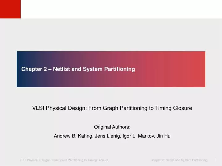
Chapter 2 – Netlist and System Partitioning VLSI Physical Design: From Graph Partitioning to Timing Closure Original Authors: Andrew B. Kahng, Jens Lienig, Igor L. Markov, Jin Hu

Chapter 2 – Netlist and System Partitioning 2.1 Introduction 2.2 Terminology 2.3 Optimization Goals 2.4 Partitioning Algorithms 2.4.1 Kernighan-Lin (KL) Algorithm 2.4.2 Extensions of the Kernighan-Lin Algorithm 2.4.3 Fiduccia-Mattheyses (FM) Algorithm 2.5 Framework for Multilevel Partitioning 2.5.1 Clustering 2.5.2 Multilevel Partitioning 2.6 System Partitioning onto Multiple FPGAs

2.1 Introduction System Specification Partitioning Architectural Design ENTITY test isport a: in bit;end ENTITY test; Functional Designand Logic Design Chip Planning Placement Circuit Design Physical Design Clock Tree Synthesis Physical Verificationand Signoff DRCLVS ERC Signal Routing Fabrication Timing Closure Packaging and Testing Chip

2.1 Introduction Circuit: Cut cb 1 3 2 7 8 4 6 5 Cut ca Block A Block B Block A Block B 5 4 1 8 3 4 1 8 5 2 7 3 2 6 6 7 Cut ca: four external connections Cut cb: two external connections

2.2 Terminology Block (Partition) Graph G1: Nodes 3, 4, 5. 4 4 1 1 6 3 5 6 5 3 2 2 Cells Graph G2: Nodes 1, 2, 6. Collection of cut edges Cut set: (1,3), (2,3), (5,6),

2.3 Optimization Goals • Given a graph G(V,E) with |V| nodes and |E| edges where each node v  V and each edge e  E. • Each node has area s(v) and each edge has cost or weight w(e). • The objective is to divide the graph G into k disjoint subgraphs such that all optimization goals are achieved and all original edge relations are respected.

2.3 Optimization Goals • In detail, what are the optimization goals? • Number of connections between partitions is minimized • Each partition meets all design constraints (size, number of external connections..) • Balance every partition as well as possible • How can we meet these goals? • Unfortunately, this problem is NP-hard • Efficient heuristics are developed in the 1970s and 1980s. They are high quality and in low-order polynomial time. 7

2.4.1 Kernighan-Lin (KL) Algorithm Given: A graph with 2n nodes where each node has the same weight. Goal: A partition (division) of the graph into two disjoint subsets A and B with minimum cut cost and |A| = |B| = n. Example: n = 4 5 1 6 2 BlockA Block B 3 7 4 8

2.4.1 Kernighan-Lin (KL) Algorithm – Terminology Cost D(v) of moving a node v D(v) = |Ec(v)| – |Enc(v)| , where Ec(v) is the set of v’s incident edges that are cut by the cut line, and Enc(v) is the set of v’s incident edges that are not cut by the cut line. High costs (D > 0) indicate that the node should move, while low costs (D < 0) indicate that the node should stay within the same partition. 5 1 6 2 3 7 Node 3: D(3) = 3-1=2 4 8 Node 7: D(7) = 2-1=1

2.4.1 Kernighan-Lin (KL) Algorithm – Terminology • Gain of swapping a pair of nodes a und b • g = D(a) + D(b) - 2* c(a,b), • where • D(a),D(b) are the respective costs of nodes a, b • c(a,b) is the connection weight between a and b: • If an edge exists between a and b, then c(a,b)= edge weight (here 1), • otherwise, c(a,b)= 0. • The gain g indicates how useful the swap between two nodes will be • The larger g, the more the total cut cost will be reduced 5 1 6 2 3 7 4 8

2.4.1 Kernighan-Lin (KL) Algorithm – Terminology Node 7: D(7) = 2-1=1 • Gain of swapping a pair of nodes a und b • g = D(a) + D(b) - 2* c(a,b), • where • D(a),D(b) are the respective costs of nodes a, b • c(a,b) is the connection weight between a and b: • If an edge exists between a and b, then c(a,b)= edge weight (here 1), • otherwise, c(a,b)= 0. 5 1 6 2 3 7 Node 3: D(3) = 3-1=2 4 8 5 1 g (3,7) = D(3) + D(7) - 2* c(a,b) = 2 + 1 – 2 = 1 6 2 => Swapping nodes 3 and 7 would reduce the cut size by 1 3 7 4 8

2.4.1 Kernighan-Lin (KL) Algorithm – Terminology Node 5: D(5) = 2-1=1 • Gain of swapping a pair of nodes a und b • g = D(a) + D(b) - 2* c(a,b), • where • D(a),D(b) are the respective costs of nodes a, b • c(a,b) is the connection weight between a and b: • If an edge exists between a and b, then c(a,b)= edge weight (here 1), • otherwise, c(a,b)= 0. 5 1 6 2 3 7 Node 3: D(3) = 3-1=2 4 8 5 1 g (3,5) = D(3) + D(5) - 2* c(a,b) = 2 + 1 – 0 = 3 6 2 => Swapping nodes 3 and 5 would reduce the cut size by 3 3 7 4 8

2.4.1 Kernighan-Lin (KL) Algorithm – Terminology Gain of swapping a pair of nodes a und b The goal is to find a pair of nodes a and b to exchange such that g is maximized and swap them.

2.4.1 Kernighan-Lin (KL) Algorithm – Terminology Maximum positive gain Gmof a pass The maximum positive gainGm corresponds to the best prefix of m swaps within the swap sequence of a given pass. These m swaps lead to the partition with the minimum cut cost encountered during the pass. Gm is computed as the sum of Δg values over the first m swaps of the pass, with m chosen such that Gm is maximized.

2.4.1 Kernighan-Lin (KL) Algorithm

2.4.1 Kernighan-Lin (KL) Algorithm – Example 5 1 6 2 3 7 4 8 Cut cost: 9 Not fixed: 1,2,3,4,5,6,7,8

2.4.1 Kernighan-Lin (KL) Algorithm – Example 5 1 6 2 3 7 4 8 Cut cost: 9 Not fixed: 1,2,3,4,5,6,7,8 Costs D(v) of each node: D(1) = 1 D(5) = 1D(2) = 1 D(6) = 2D(3) = 2 D(7) = 1D(4) = 1 D(8) = 1 Nodes that lead to maximum gain

2.4.1 Kernighan-Lin (KL) Algorithm – Example 5 1 6 2 3 7 4 8 Cut cost: 9 Not fixed: 1,2,3,4,5,6,7,8 Costs D(v) of each node: D(1) = 1 D(5) = 1D(2) = 1 D(6) = 2D(3) = 2D(7) = 1D(4) = 1 D(8) = 1g1 = 2+1-0 = 3 Swap (3,5) G1 = g1 =3 Nodes that lead to maximum gain Gain after node swapping Gain in the current pass

2.4.1 Kernighan-Lin (KL) Algorithm – Example 5 5 1 1 6 6 2 2 3 7 3 7 4 4 8 8 Cut cost: 9 Not fixed: 1,2,3,4,5,6,7,8 D(1) = 1 D(5) = 1D(2) = 1 D(6) = 2D(3) = 2D(7) = 1D(4) = 1 D(8) = 1g1 = 2+1-0 = 3 Swap (3,5) G1 = g1 =3 Nodes that lead to maximum gain Gain after node swapping Gain in the current pass

2.4.1 Kernighan-Lin (KL) Algorithm – Example 5 5 1 1 6 6 2 2 3 7 3 7 4 4 8 8 Cut cost: 9 Not fixed: 1,2,3,4,5,6,7,8 Cut cost: 6 Not fixed: 1,2,4,6,7,8 D(1) = 1 D(5) = 1D(2) = 1 D(6) = 2D(3) = 2D(7) = 1D(4) = 1 D(8) = 1g1 = 2+1-0 = 3 Swap (3,5) G1 = g1 =3

2.4.1 Kernighan-Lin (KL) Algorithm – Example 5 5 1 1 6 6 2 2 3 7 3 7 4 4 8 8 Cut cost: 9 Not fixed: 1,2,3,4,5,6,7,8 Cut cost: 6 Not fixed: 1,2,4,6,7,8 D(1) = 1 D(5) = 1D(2) = 1 D(6) = 2D(3) = 2D(7) = 1D(4) = 1 D(8) = 1g1 = 2+1-0 = 3 Swap (3,5) G1 = g1 =3 D(1) = -1 D(6) = 2D(2) = -1 D(7)=-1D(4) = 3D(8)=-1

2.4.1 Kernighan-Lin (KL) Algorithm – Example 5 5 5 1 1 1 6 6 6 2 2 2 3 7 3 7 3 7 4 4 4 8 8 8 Cut cost: 9 Not fixed: 1,2,3,4,5,6,7,8 Cut cost: 6 Not fixed: 1,2,4,6,7,8 D(1) = 1 D(5) = 1D(2) = 1 D(6) = 2D(3) = 2D(7) = 1D(4) = 1 D(8) = 1g1 = 2+1-0 = 3 Swap (3,5) G1 = g1 =3 D(1) = -1 D(6) = 2D(2) = -1 D(7)=-1D(4) = 3D(8)=-1g2 = 3+2-0 = 5 Swap (4,6) G2 = G1+g2=8 Nodes that lead to maximum gain Gain after node swapping Gain in the current pass

2.4.1 Kernighan-Lin (KL) Algorithm – Example Nodes that lead to maximum gain 5 5 5 5 1 1 1 1 6 6 6 6 2 2 2 2 3 7 3 7 3 7 3 7 4 4 4 4 8 8 8 8 Cut cost: 9 Not fixed: 1,2,3,4,5,6,7,8 Cut cost: 6 Not fixed: 1,2,4,6,7,8 Cut cost: 1 Not fixed: 1,2,7,8 Cut cost: 7 Not fixed: 2,8 D(1) = 1 D(5) = 1D(2) = 1 D(6) = 2D(3) = 2D(7) = 1D(4) = 1 D(8) = 1g1 = 2+1-0 = 3 Swap (3,5) G1 = g1 =3 D(1) = -1 D(6) = 2D(2) = -1 D(7)=-1D(4) = 3D(8)=-1g2 = 3+2-0 = 5 Swap (4,6) G2 = G1+g2=8 D(1) = -3D(7)=-3D(2) = -3 D(8)=-3g3 = -3-3-0 = -6 Swap (1,7) G3= G2+g3= 2 Gain after node swapping Gain in the current pass

2.4.1 Kernighan-Lin (KL) Algorithm – Example 5 5 5 5 5 1 1 1 1 1 6 6 6 6 2 6 2 2 2 2 3 7 3 7 3 7 3 7 3 7 4 4 4 4 4 8 8 8 8 8 Cut cost: 9 Not fixed: 1,2,3,4,5,6,7,8 Cut cost: 6 Not fixed: 1,2,4,6,7,8 Cut cost: 1 Not fixed: 1,2,7,8 Cut cost: 7 Not fixed: 2,8 Cut cost: 9 Not fixed: – D(1) = 1 D(5) = 1D(2) = 1 D(6) = 2D(3) = 2D(7) = 1D(4) = 1 D(8) = 1g1 = 2+1-0 = 3 Swap (3,5) G1 = g1 =3 D(1) = -1 D(6) = 2D(2) = -1 D(7)=-1D(4) = 3D(8)=-1g2 = 3+2-0 = 5 Swap (4,6) G2 = G1+g2=8 D(1) = -3D(7)=-3D(2) = -3 D(8)=-3g3 = -3-3-0 = -6 Swap (1,7) G3= G2+g3= 2 D(2) = -1D(8)=-1 g4 = -1-1-0 = -2 Swap (2,8) G4 = G3+g4 = 0

2.4.1 Kernighan-Lin (KL) Algorithm – Example D(1) = 1 D(5) = 1D(2) = 1 D(6) = 2D(3) = 2D(7) = 1D(4) = 1 D(8) = 1g1 = 2+1-0 = 3 Swap (3,5) G1 = g1 =3 D(1) = -1 D(6) = 2D(2) = -1 D(7)=-1D(4) = 3D(8)=-1g2 = 3+2-0 = 5 Swap (4,6) G2 = G1+g2=8 D(1) = -3D(7)=-3D(2) = -3 D(8)=-3g3 = -3-3-0 = -6 Swap (1,7) G3= G2+g3= 2 D(2) = -1D(8)=-1 g4 = -1-1-0 = -2 Swap (2,8) G4 = G3+g4 = 0 Maximum positive gain Gm = 8 with m = 2.

2.4.1 Kernighan-Lin (KL) Algorithm – Example D(1) = 1 D(5) = 1D(2) = 1 D(6) = 2D(3) = 2D(7) = 1D(4) = 1 D(8) = 1g1 = 2+1-0 = 3 Swap (3,5) G1 = g1 =3 D(1) = -1 D(6) = 2D(2) = -1 D(7)=-1D(4) = 3D(8)=-1g2 = 3+2-0 = 5 Swap (4,6) G2 = G1+g2=8 D(1) = -3D(7)=-3D(2) = -3 D(8)=-3g3 = -3-3-0 = -6 Swap (1,7) G3= G2+g3= 2 D(2) = -1D(8)=-1 g4 = -1-1-0 = -2 Swap (2,8) G4 = G3+g4 = 0 Maximum positive gain Gm = 8 with m = 2. 5 1 Since Gm> 0,the first m = 2 swaps (3,5) and (4,6) are executed. 6 2 3 7 Since Gm> 0, more passes are needed until Gm 0. 4 8

2.4.2 Extended Kernighan-Lin (KL) Algorithm • Unequal partition sizes • Apply the KL algorithm with only min(|A|,|B|) pairs swapped • Unequal cell sizes or unequal node weights • assign a unit area, i.e. the greatest common divisor of all cell areas • k-way partitioning (generating k partitions) • Apply the KL 2-way partitioning algorithm to all possible pairs of partitions 28

2.4.3 Fiduccia-Mattheyses (FM) Algorithm • Single cells are moved independently instead of swapping pairs of cells. Thus, this algorithm is applicable to partitions of unequal size or the presence of initially fixed cells. • Cut costs are extended to include hypergraphs, i.e., nets with two or more pins. While the KL algorithm aims to minimize cut costs based on edges, the FM algorithm minimizes cut costs based on nets. • The area of each individual cell is taken into account. • Nodes and subgraphs are referred to as cells and blocks, respectively.

2.4.3 Fiduccia-Mattheyses (FM) Algorithm Given: a graph G(V,E) with nodes and weighted edges Goal: to assign all nodes to disjoint partitions, so as to minimize the total cost (weight) of all cut nets while satisfying partition size constraints

2.4.3 Fiduccia-Mattheyses (FM) Algorithm – Terminology Gain g(c) for cell c g(c) = FS(c) – TE(c) , where the “moving force“ FS(c) is the number of nets connected to c but not connected to any other cells within c’s partition, i.e., cut nets that connect only to c, and the “retention force“ TE(c) is the number of uncut nets connected to c. The higher the gain g(c), the higher is the priority to move the cell c to the other partition. 3 2 b e a 4 c d 1 5 Cell 2: FS(2) = 0 TE(2) = 1 g(2) = -1

2.4.3 Fiduccia-Mattheyses (FM) Algorithm – Terminology Gain g(c) for cell c g(c) = FS(c) – TE(c) , where the “moving force“ FS(c) is the number of nets connected to c but not connected to any other cells within c’s partition, i.e., cut nets that connect only to c, and the “retention force“ TE(c) is the number of uncut nets connected to c. 3 2 b e a 4 c d 1 5 3 2 Cell 1: FS(1) = 2 TE(1) = 1 g(1) = 1 Cell 2: FS(2) = 0 TE(2) = 1 g(2) = -1 Cell 3: FS(3) = 1 TE(3) = 1 g(3) = 0 Cell 4: FS(4) = 1 TE(4) = 1 g(4) = 0 Cell 5: FS(5) = 1 TE(5) = 0 g(5) = 1 b e a 4 c d 1 5

2.4.3 Fiduccia-Mattheyses (FM) Algorithm – Terminology Maximum positive gain Gmof a pass The maximum positive gain Gm is the cumulative cell gain of m moves that produce a minimum cut cost. Gmis determined by the maximum sum of cell gains g over a prefix of m moves in a pass

2.4.3 Fiduccia-Mattheyses (FM) Algorithm – Terminology Ratio factor The ratio factor is the relative balance between the two partitions with respect to cell area. It is used to prevent all cells from clustering into one partition. The ratio factor r is defined as where area(A) and area(B) are the total respective areas of partitions A and B

2.4.3 Fiduccia-Mattheyses (FM) Algorithm – Terminology Balance criterion The balance criterionenforces the ratio factor. To ensure feasibility, the maximum cell area areamax(V) must be taken into account. A partitioning of V into two partitions A and B is said to be balanced if [ r ∙ area(V) – areamax(V) ] ≤ area(A) ≤ [ r ∙ area(V) + areamax(V) ]

2.4.3 Fiduccia-Mattheyses (FM) Algorithm – Terminology Base cell A base cell is a cell c that has maximum cell gain g(c) among all free cells, and whose move does not violate the balance criterion. Base cell Cell 1: FS(1) = 2 TE(1) = 1 g(1) = 1 Cell 2: FS(2) = 0 TE(2) = 1 g(2) = -1 Cell 3: FS(3) = 1 TE(3) = 1 g(3) = 0 Cell 4: FS(4) = 1 TE(4) = 1 g(4) = 0

2.4.3 Fiduccia-Mattheyses (FM) Algorithm

2.4.3 Fiduccia-Mattheyses (FM) Algorithm – Example 3 2 A B Given:Ratio factor r = 0,375 area(Cell_1) = 2 area(Cell_2) = 4 area(Cell_3) = 1 area(Cell_4) = 4 area(Cell_5) = 5. b e a 4 c d 1 5 Step 0: Compute the balance criterion [ r ∙ area(V) – areamax(V) ] ≤ area(A) ≤ [ r ∙ area(V) + areamax(V) ] 0,375 * 16 – 5 = 1 area(A)  11 = 0,375 * 16 +5.

2.4.3 Fiduccia-Mattheyses (FM) Algorithm – Example 3 2 A B b e a 4 c d 1 5 Step 1:Compute the gains of each cell Cell 1: FS(Cell_1) = 2 TE(Cell_1) = 1 g(Cell_1) = 1 Cell 2: FS(Cell_2) = 0 TE(Cell_2) = 1 g(Cell_2) = -1 Cell 3: FS(Cell_3) = 1 TE(Cell_3) = 1 g(Cell_3) = 0 Cell 4: FS(Cell_4) = 1 TE(Cell_4) = 1 g(Cell_4) = 0 Cell 5: FS(Cell_5) = 1 TE(Cell_5) = 0 g(Cell_5) = 1

2.4.3 Fiduccia-Mattheyses (FM) Algorithm – Example 3 2 A B Cell1: FS(Cell_1) = 2 TE(Cell_1) = 1 g(Cell_1) = 1 Cell 2: FS(Cell_2) = 0 TE(Cell_2) = 1 g(Cell_2) = -1 Cell 3: FS(Cell_3) = 1 TE(Cell_3) = 1 g(Cell_3) = 0 Cell 4: FS(Cell_4) = 1 TE(Cell_4) = 1 g(Cell_4) = 0 Cell 5: FS(Cell_5) = 1 TE(Cell_5) = 0 g(Cell_5) = 1 b e a 4 c d 1 5 Step 2:Select the base cell Possible base cells are Cell 1 and Cell 5 Balance criterion after moving Cell 1: area(A) = area(Cell_2) = 4 Balance criterion after moving Cell 5: area(A) = area(Cell_1) + area(Cell_2) + area(Cell_5) = 11 Both moves respect the balance criterion, but Cell 1 is selected, moved, and fixed as a result of the tie-breaking criterion.

2.4.3 Fiduccia-Mattheyses (FM) Algorithm – Example 3 2 A B b e a 4 c d 1 5 Step 3: Fix base cell, update g values Cell 2: FS(Cell_2) = 2 TE(Cell_2) = 0 g(Cell_2) = 2 Cell 3: FS(Cell_3) = 0 TE(Cell_3) = 1 g(Cell_3) = -1 Cell 4: FS(Cell_4) = 0 TE(Cell_4) = 2 g(Cell_4) = -2 Cell 5: FS(Cell_5) = 0 TE(Cell_5) = 1 g(Cell_5) = -1 After Iteration i = 1:Partition A1 = 2, Partition B1 = 1,3,4,5, with fixed cell 1.

2.4.3 Fiduccia-Mattheyses (FM) Algorithm – Example Iteration i = 1 3 2 A B Cell 2: FS(Cell_2) = 2 TE(Cell_2) = 0 g(Cell_2) = 2 Cell 3: FS(Cell_3) = 0 TE(Cell_3) = 1 g(Cell_3) = -1 Cell 4: FS(Cell_4) = 0 TE(Cell_4) = 2 g(Cell_4) = -2 Cell 5: FS(Cell_5) = 0 TE(Cell_5) = 1 g(Cell_5) = -1 b e a 4 c d 1 5 Iteration i = 2 Cell 2 has maximum gain g2 = 2, area(A) = 0, balance criterion is violated. Cell 3 has next maximum gain g2 = -1, area(A) = 5, balance criterion is met. Cell 5 has next maximum gain g2= -1, area(A) = 9, balance criterion is met. Move cell 3, updated partitions: A2 = {2,3}, B2 = {1,4,5}, with fixed cells {1,3}

2.4.3 Fiduccia-Mattheyses (FM) Algorithm – Example Iteration i = 2 3 2 A Cell 2: g(Cell_2) = 1 Cell 4: g(Cell_4) = 0 Cell 5: g(Cell_5) = -1 e B b a 4 c d 1 5 Iteration i = 3 Cell 2 has maximum gain g3 = 1, area(A) = 1, balance criterion is met.Move cell 2, updated partitions: A3 = {3}, B3 = {1,2,4,5}, with fixed cells {1,2,3}

2.4.3 Fiduccia-Mattheyses (FM) Algorithm – Example Iteration i = 3 3 2 B A e Cell 4: g(Cell_4) = 0 Cell 5: g(Cell_5) = -1 b a 4 c d 1 5 Iteration i = 4 Cell 4 has maximum gain g4 = 0, area(A) = 5, balance criterion is met.Move cell 4, updated partitions: A4 = {3,4}, B3 = {1,2,5}, with fixed cells {1,2,3,4}

2.4.3 Fiduccia-Mattheyses (FM) Algorithm – Example Iteration i = 4 3 2 B A e Cell 5: g(Cell_5) = -1 b a 4 c d 1 5 Iteration i = 5 Cell 5 has maximum gain g5 = -1, area(A) = 10, balance criterion is met.Move cell 5, updated partitions: A4 = {3,4,5}, B3 = {1,2}, all cells {1,2,3,4,5} fixed.

2.4.3 Fiduccia-Mattheyses (FM) Algorithm – Example 3 2 B A e b a 4 c d 1 5 Step 5: Find best move sequence c1 … cm G1 = g1 = 1G2 = g1 + g2 = 0G3 = g1 + g2 + g3 = 1G4 = g1 + g2 + g3 + g4 = 1G5 = g1 + g2 + g3 + g4 + g5 = 0. Maximum positive cumulative gain found in iterations 1, 3 and 4. The move prefix m = 4 is selected due to the better balance ratio (area(A) = 5); the four cells 1, 2, 3and 4 are then moved. Result of Pass 1: Current partitions: A = {3,4}, B = {1,2,5}, cut cost reduced from 3 to 2.

Chapter 2 Supplemental: Difference between KL & FM • Component dependency of partitioning algorithms • KL is based on the number of edges • FM is based on the number of nets • Time complexity of partitioning algorithms • KL has cubic time complexity • FM has linear time complexity 47

2.5.1 Clustering • To make things easy, groups of tightly-connected nodes can be clustered, absorbing connections between these nodes • Size of each cluster is often limited so as to prevent degenerate clustering, i.e. a single large cluster dominates other clusters • Refinement should satisfy balance criteria 49

Chapter 2 – Netlist and System Partitioning