Download
1 / 56
560 likes | 651 Vues
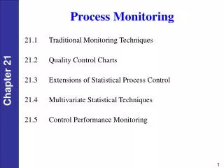
KE-90.5100 Process Monitoring (4cr). Course information. The course consists of Lectures: Tue 14 – 16, Ke3 Thu 12 – 14, Ke3 Exercises: Fri 10:00 – 12:00, computer class room Exam: Oct 31 2008 Jan 8 2009. Course information. The course consists of

E N D
Course information • The course consists of • Lectures: • Tue 14 – 16, Ke3 • Thu 12 – 14, Ke3 • Exercises: • Fri 10:00 – 12:00, computer class room • Exam: • Oct 31 2008 • Jan 8 2009
Course information • The course consists of • 5 obligatory homeworks (presented during exercises): • Assistant: M.Sc. Cheng Hui • submit report by email within 2 weeks (di.zhang@tkk.fi) • All exercises have to be OK before exam • Assignments: Group work to be presented at the end of the course • The grade consists of • Assignment (30%) • Exam (70%)
Course material • Course web pages • Slides • Handouts • Exercises/Homework • Material from assignment
Course Staff • Hui Cheng, hui.cheng@hut.fi, reception Thu 10 –11, F302 • Alexey Zakharov • Fernando Dorado • Di Zhang
Scope of the course Tools of the process control engineer Classical Control -PID -Bode, -Nyqvist -… Modern Control - Multivariable control - MPC - IMC -… Intelligent methods - Neural Networks - Fuzzy logic - GA • Multivariate data analysis • PCA • PLS • SOM • Modeling and • simulation • - First principles • modeling • - Identification • Simulation of • dynamic systems • - … KE-90.2100 Basics of process automation KE-90.5100 Process Monitoring KE-90.4510 Control applications in process industries KE-90.3100 Process Modelling and Simulation
Scope of the course • After the course you will know • How and when to use some statistical process monitoring methods • The basics of neural networks and fuzzy systems and how to utilize them in monitoring and control • The basics of genetic algorithms
Introduction • The idea of process monitoring • Goals of process monitoring • The process monitoring loop • Process monitoring methods • Data selection • Data pretreatment • Univariate vs. multivariate statistics
The idea To monitor or monitoring generally means to be aware of the state of a system
The idea • Multivariate data in industrial processes: impossible for human operator to monitor hundreds of measurements for possible faults • Costs and safety issues with equipment malfunctions / process disturbances • Shutdowns expensive • Amount of maintenance breaks • New equipment: delivery time • Safe working environment for plant staff
The idea • Process equipment malfunctions and process disturbances • E.g. contamination of sensors, faults of analyzers, clogging of filters, degradation of catalyst, changing properties of feed stock, leaks, actuator faults etc… • How to detect early enough? • How to distinguish between?
The goals Get indication of • process disturbances and • malfunctions in process equipment As early as possible to • Increase uniform quality of the products • Improve safety • Minimize maintenance costs
The process monitoring loop no Fault Identification Process Recovery Fault Diagnosis Fault Detection yes Fault Detection = determining whether a fault has occurred Fault Identification = identifying the variables most relevant for diagnosing the fault Fault Diagnosis = determining which fault occurred Process Recovery = Removing the effect of the fault
Process monitoring methods Process monitoring + Easier to implement − Don’t include process knowledge + Includes process knowledge − Needs process models Model-Based Data-Based Quantitative Qualitative Statistical Neural Networks
Model-Based Residual based observers Parity-space based Causal models Signed digraphs Statistical PCA PLS RPCA Process monitoring methods Process monitoring Data-Based Quantitative Qualitative Trend analysis Rule-based Neural Networks introductory Scope of the course PCA PLS RPCA.. SOM MLP RBFN.. + GA and some Control
Data selection • Training data includes: • If goal is to verify that process is in normal state (monitoring) the process data used for training should represent normal conditions • If the goal is to identify if the process is in a normal or some specified faulty state the process data used for training should include all the possible faulty states as well as the normal state • Testing data • Completely independent from training data!
Data pretreatment • Main procedures in pretreatment are: • Removing variables • The data set may contain variables that have no relevant information for monitoring • Removing outliers • Outliers are isolated measurement values that are erroneous and will cause biased parameter estimates for the method used. Methods for removing outliers include visual inspection and statistical tests. • Autoscaling • Process data often needs to be scaled to avoid particular variables dominating the process monitoring method (autoscaling = subtract mean and divide by standard deviation)
out-of-control in-control upper control limit target lower control limit Univariate vs. multivariate statistics • The most simple type of monitoring is based on univariate statistics • Individual thresholds are determined for each variable (Shewart charts)
Univariate vs. multivariate statistics • Tight thresholds result in a high false alarm rate but low missed alarm rate • Limits too spread apart result in low false alarm rates but high missed alarm rates • A trade off between false alarms and missed alarms normal faulty threshold false alarms missed alarms
Univariate vs. multivariate statistics • Univariate methods determine threshold for each variable individually without considering other variables • The fact that there are correlations between the variables is ignored • The multivariate T2 statistic takes into account these correlations • The T2 statistic is based on an eigenvector decompostion of the covariance matrix
Univariate vs. multivariate statistics • Comparison of univariate statistics and T2 statistic x2 T2 statistical confidence region Abnormal data can be classified as ok! x1 univariate statistical confidence region More on T2 later in the PCA part
Principal Component Analysis Process monitoring Model-Based Data-Based Quantitative Qualitative Statistical Neural Networks PCA
Principal component analysis • Linear method • Greatly reduces the number of variables to be monitored – data compression • Based on eigenvalue and eigenvector decomposition of the covariance matrix • Simple indexes for monitoring
PCA model PC2 x2 PC1 PC1: Direction of largest variation PC2: Direction of 2. largest variation x1 Principal component analysis • The idea of PCA is to form a minimum number of new variables to describe the variation of the data by using linear combinations of the original variables
PC2 x2 PCA PC1 x1 PCA- principal components • The new axes = principal components are selected according to the direction of highest variation in the original data set • The new axes are orthogonal
PCA- principal components • Principal components will rotate the data set so that the different groups might be separable Separation of faulty data on pc2-axis No separation of faulty data (red) with original axis pc2 x2 pc1 x1
PCA- scores • The PCA scores are the values of the original data points on the principal component axes PC2 Sample 1 PC1
PCA model calculation • The direction of the principal components = eigenvectors • The variation of the data along a eigenvector is given by the corresponding eigenvalue x2 PC1=e1=w11x1+w12x2 PCA model x1
Principal component analysis • Principal Component Analysis is based on a eigenvalue/eigenvector decomposition of the covariance matrix of the data set (X) with n observations (rows) and m variables (columns). X is centered to have zero mean and scaled so that each variable has the same variance (especially if the variables have different units Covariance matrix C The covariance matrix can be decomposed:
Principal component analysis • The decomposition can be done by solving • In Matlab the eigenvalues and eigenvectors are obtained by: [eig_vec,eig_val] = eig(C) • Each eigenvector is a column in eig_vec and the eigenvalues are on the diagonal of eig_val • A score-matrix T can be calculated: T = XVk • Vk is a transformation matrix containing the eigenvectors corresponding to the k largest eigenvalues. The user chooses k (more later) • T is a ”compressed” version of X and
Principal component analysis • The compressed data can be decompressed: • There is a residual matrix E between the original data and the decompressed data • Combining the equations and rewriting the TVkT term: • pi are the principal components • The scores ti are the distances along the principal component pi
Principal component analysis • Matlab demo: Compressing and decompressing data via eigenvalue decomposition
Principal Component Analysis • Example: Calculate (by hand) the eigenvalues and eigenvectors for: Specify that also verify Recall that
Monitoring indexes • SPE – variation outside the model, distance off the model plane • Hotelling T2 – variation inside the model, distance from the origin along the model plane Points with SPE violation SPE Points with T2 violation PC2 PCA model plane PC1
Monitoring indexes • T2: Measures systematic variations of the process. For individual observation: • SPE: Measures the random variations of the process
Different view SPE
Monitoring indexes • The process can be also monitored by tracking the score values for each principal component
PCA - calculate the model • Zero-mean the original data set. • Compute the covariance matrix C • Compute the eigenvalues and eigenvectors. Modify the matrices so, that the eigenvalues are in decreasing order (remember to do the same operations to the eigenvectors) • Choose how many principal components to use. (Plot eigenvalues, captured variance) • Form the transformation matrix Vk (principal components) and eigenvalue matrix Λk. • Compute confidence limits for the scores of every PC • Compute the Hotelling T2 & SPE limits
PCA - calculate the model • Scale the original data set X (zero-mean, unit variance if necessary). • Calculate the covariance matrix
PCA - calculate the model • Compute the eigenvalues and eigenvectors. The eigenvalues are computed according to The eigenvectors can be solved from the equation: Remember to keep the eigenvectors in the same order as the eigenvalues
PCA - calculate the model 4. Choose how many principal components to use. (Plot eigenvalues, captured variance)
PCA - calculate the model With 7 PCs 96% of the variance is captured
PCA - calculate the model • Form the transformation matrix Vk (eigenvectors) and eigenvalue matrix ΛK .
PCA - calculate the model 6. Compute confidence limits for the scores of every PC sqrt(lamda)*tinv(alfa+(1-alfa)/2,N-1) In Matlab: α α = confidence level
PCA - calculate the model 7. Compute Hotelling T2 limit & SPE limit where the F(K,N-K,) corresponds to the probability point on the F-distribution with (K,N-K) degrees of freedom and confidence level . N = # of data samples, K = # of PCs “Unused” eigenvalues where m= number of original variables, k=number of principal components in the model, cα= upper limit from normal distribution with conf. level α
PCA – the new data • Scale the new data set with training data scaling values . • Compute PCA transformation (i.e. scores for all the chosen principal components) using Vk. • Compare the scores to confidence limits. If inside the limits, then OK. • Compute the Hotelling T2 & SPE values for the new data set • Compare the Hotelling T2 & SPE values to the limits. If under the limit, then OK
PCA – the new data • Scale the new data set with training data scaling values • Compute PCA transformation (i.e. scores for all the chosen principal components) using Vk.
PCA – the new data 3. Compare the scores to confidence limits. If inside the limits, then OK 4. Compute the Hotelling T2 & SPE values for the new data set 5. Compare the Hotelling T2 & SPE values to the limits. If under the limit, then OK
Fault identification • Once a fault has been detected, the next step is determine the cause of the out-of-control status • One way to handle this is by using so called contribution plots
Contribution plots • In response to T2 violations we can obtain contribution plots according to: • For observation xi, find the r cases when the normalized scores ti2/λi > T2/a • Calculate the contribution of each variable xj to the out-of-control scores ti • When conti,j is negative set it equal to zero • Calculate the total contribution of the jth process variable • Plot CONTj for all process variables in a single plot