Download
1 / 21
210 likes | 302 Vues
Additive Distances Between DNA S equences. 1. 3. 2. C. G. T. A. A C. C C. 1. Additive Evolutionary distance : The number of substitutions which occurred during the sequence evolution. substitutions. site 1. site 2. site 3. 0.

E N D
Additive DistancesBetween DNA Sequences MPI, June 2012
1 3 2 C G T A A C C C 1 Additive Evolutionary distance :The number of substitutions which occurred during the sequence evolution substitutions site 1 site 2 site 3 0 Some substitutions are hidden, due to overwriting. Therefore, the exact number of subst. is usually larger than the number of observed changes.
Edge weight = Expected number of substit’s per site u Number of substitutions per site 0.321 v MPI, June 2012
Interleaf distances: sum of edge weights v u d(u,v) = 1.12 0.3 0.5 0.42 When the exact number of substitutions between any two sequences is known, NJ (and any other algorithm which reconstructs trees from the exact distances) returns the correct evolutionary tree.
Estimating# of substitutionsfrom observed substitutionsrequiresSubstitution Model JC [Jukes Cantor 1969] Kimura 2 Parameter (K2P) [Kimura 1980] HKY [Hasegawa, Kishino and Yano 1985] TN [Tamura and Nei 1993] GTR: Generalised time-reversible [Tavaré 1986] …and more…
Jukes Cantor model:All substitutions are equally like JC generic rate matrix tis the expected # of substitutions per site u tuv Ruv = v
Rate Matrix R R = (Theory of Markov Processes) Substitution Matrix P P =
JC distance estimation:First estimate the substitution matrix anEstimationof Puv From observed substit’s
Estimatet from estimation of p(t)by “reverse engineering” Solve the formula for p(t)
Checking the effectof estimation-errorsin Reconstructing Quartets
Quartets Reconstruction = Finding the correct split Quartets are trees with four leaves. They have three possible (fully resolved) topologies, called splits: A C A B A C B D C D B D Distance methods resolves splits by the 4 point method
wsep The 4 points method A C B D The 4-point condition: The 4-point condition for estimated distances:
Evaluate the accuracy ofreconstructing quartetsusing evolutionary distances root t is “evolutionary time” The diameter of the quartet is 22t D A C B
Phase A: simulate evolution D A C B
ç ÷ ç ÷ Apply the 4p condition. Is the recontruction correct? ç ÷ ç ÷ ç ÷ ç ÷ ç ÷ ç ÷ è ø D C A B Phase B: reconstruct the split by the 4p condition compute distances between sequences, Repeat this process 10,000 times, count number of failures
This test was applied on the model quartet with various diameters … … • For each diameter, mark the fraction (percentage) of the simulations in which the reconstruction failed (next slide)
Performance of K2P distances in resolving quartets, small diameters: 0.01-0.2 Template quartet
“site saturation” Performance for larger diameters
Repeat this experiment on the Hasegawa tree • Assume the JC model. • Reconstruct by the NJ algorithm (use any variants of NJ available in MATLAB)