Download
1 / 43
430 likes | 664 Vues
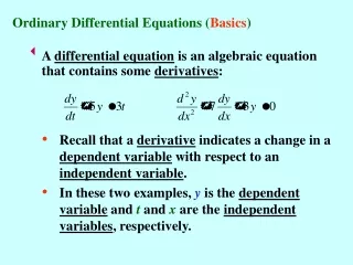
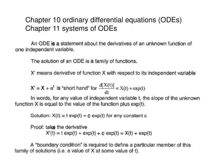
Chapter 10 ordinary differential equations (ODEs) Chapter 11 systems of ODEs. System of ODEs. Initial value problems. Regardless of problem statement, identify f(x,t), a, b, and X(a). Initial-value problem: X’ = f(X, t); X(t 0 ) = X 0. Solved by “separation of variables”.

E N D
Chapter 10 ordinary differential equations (ODEs) Chapter 11 systems of ODEs
Initial value problems Regardless of problem statement, identify f(x,t), a, b, and X(a)
Initial-value problem: X’ = f(X, t); X(t0) = X0 Solved by “separation of variables”
Taylor-series method Given 2 types of error truncation error round-off error
Higher-order Taylor series methods x’(t) has both explicit and implicit time dependence given Given the value of x at t=1 evaluate x’(1), x’’(1), x’’’(1), etc. →x(1+h) = x(1)+hx’(1)+h2x’’(1)/2… then evaluate x’(1+h), x’’(1+h), x’’’(1+h), etc. → x(1+2h) = x(1+h)+…
Components of MatLab code to solve initial value problems main solver encoder Solver: advances table X(t) → X(t+h), estimates local truncation error, controls propagation of error, etc. Is independent of a particular ODE Encoder: Tells solver how to calculate X’(t) for a particular ODE To solve a single ODE, encoder passed to solver as function handle For systems of ODEs, encoder passed to solver as an m-file Main: Defines initial conditions and domain of solution Sets solver parameters (number of points, error tolerance, etc. Calls solver for the particular ODE , analyze the results Exception: In higher-order Taylor method, encoder is part of solver
Advantages of MatLab’s decomposition of problem: functions are specialized main solver encoder Solver: can be developed by criterion of table accuracy only, no concern for particular ODE or user objectives Encoder: only function is to tells the solver how to calculate X’(t) for all of the unknown functions in the problem. Encoder can be as simple as an inline function definition (one unknown) or as complex as an m-file describing a system being modeled by thousands of coupled ODEs Main: function restricted to problem setup (introduce encoder to solver) and downstream processing. Small changes for different problems
Develop approach for Euler method x(t+h) = x(t) + hx’(t, x(t)) main solver encoder Start by developing the solver For singe ODE encoder = inline function Write main to get results you need
main MatLab code 4th order Taylor-series method solver encoder Command window function definition specific to problem derivatives calculated in order nested form saves operations No reason why driver and function should be separate See pseudo-code text p434
Problems 10.1-10 and 10.1-11 p437 x’ = t2 + x3 5 equations needed for 4th order Taylor x’ = x + ex 5 equations needed for 4th order Taylor x’ = x2 – cos(x) 6 equations needed for 5th order
Runge-Kutta method: x’(t) = f(t, x(t)) x(t0) = x0 Find method as accurate as Taylor series that does not involve higher order derivatives. 2nd order Runge-Kutta: Look for solution of the form x(t + h) = x(t) + w1F1 + w2F2 where F1 = h f(t, x(t)) F2 = h f(t +ah, x + bF1). Note: h in definition of F1 and F2 so they have the same units as x. All 4 parameters, w1, w2, a, and b are dimensionless
Look for solution of the form x(t + h) = x(t) + w1F1 + w2F2 where F1 = h f(t, x(t)) F2 = h f(t +ah, x + bF1) Expanding f(t +ah, x + bF1) to 1st order in h give x(t+h) to 2nd order in h
Note: F1 alone is Euler’s method Pseudo-code text p443
Runge-Kutta-Fehlberg Method Evaluate both 4th and 5th order Runge Kutta Use difference as estimate of error Adjust h to keep error in bounds
Inside a loop to generate a table of values of X(t) Basic idea behind MatLabs ODE45
MatLab’s ODE45 solver Encoder is inline function. Specify domain of solution. ODE45 chooses points Plot results Display number of points Compare last value in table to exact
337 unequally spaced point X(10) correct to 4 signicant figures
Assignment 6 due 3/6/14 main solver encoder Use the design above to implement Euler, RK2, RK4, and ODE45 methods to solve x’ = 1 + x2 + t3 for x(2) given x(1) = -4 Compare, by percent difference, your values with the accurate value on p434 of text. Hand in your solvers and copy of command window where solver is called
Predictor-Corrector Methods: At every value of t, predict Xp(t+h) Use Xp(t+h) to get more accurate X(t+h) Example: Improved Euler (p10.1-15 p437) Xp(t+h) = X(t) + hX’(t,X(t)) (normal Euler) X(t+h) = X(t) + h[X’(t,X(t))+X’(t+h, Xp(t+h))]/2 Is this the same as RK2?
Adams-Bashforth-Moulton (ABM) method Both sides of equation depend on X(t)
Derive a correction to value at t+h “predictor-corrector” method
Systems of ODEs Solved by Taylor, RK and ODE45
Use the Taylor series method to solve the the system x’ = -3y y’ = x/3
Taylor series method applied to system x’ = -3y y’ = x/3
Euler’s method applied to system of ODEs Similar coding allows RK4 to be applied to systems of ODEs
Compare Eulersys with exact Essentially the same for RK4 Also works for RK4
Compare vecEulersys with exact Note: neqs is not used Vectorize Eulersys Similarly for vecRK4
ODE45 applied to system of ODEs Encoder in m-file called xpsys_cp2_p775_CK6
ODE45 solution for system x’ = t +x2 – y y’ = t2 – x+y2 x(0) = 3, y(0) = 2 Very rapid change in solution →
Assignment 7 Due 3/13/2014: Solve the system of equations x’=x – y + 2t - t2 - t3 y’=x + y - 4t2 + t3 for 0 < t < 1 subject to the initial condition x(0)=1, y(0)=0 using the following: Euler’s method 4th order Runge-Kutta method MATLAB’s ode45 solver For each method, make a plot that compares your result to the exact solution x(t)=exp(t)cos(t) + t2 y(t)=exp(t)sin(t) - t3 Each plot must distinguish numerical from exact solution.
Suggested problems from the text on ODEs Chapter 10.1 p436: Taylor series Problems 1a, 1b, 1e, 2a, 2b, 5, 10, 11a Computer problems 1, 2, 8, 9, 10 Chapter 10.2 p445: RK4 single ODE Problems 1, 2, 5, 6 Computer problems 1, 2, 4, 6, 10, 12 Chapter 11.1 p475: RK4 system of ODEs Computer problems 3, 5, 6, 7
RK solver for system of ODEs: number = neqs 1st row of y contains initial values Each column of y is solution of one of the unknowns Build solution matrix row-by-row Encoder xpsys returns x’(t)=f(t,x) for system