Download
1 / 41
410 likes | 527 Vues
The Effects of Lake Michigan on Mature Mesoscale Convective Systems. Nicholas D. Metz and Lance F. Bosart Department of Atmospheric and Environmental Sciences University at Albany/SUNY, Albany, NY 12222 E-mail: nmetz@atmos.albany.edu Support provided by the NSF ATM–0646907

E N D
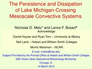
The Effects of Lake Michigan on Mature Mesoscale Convective Systems Nicholas D. Metz and Lance F. Bosart Department of Atmospheric and Environmental Sciences University at Albany/SUNY, Albany, NY 12222 E-mail: nmetz@atmos.albany.edu Support provided by the NSF ATM–0646907 18th Great Lakes Operational Meteorology Workshop Toronto, Ontario 23 March 2010
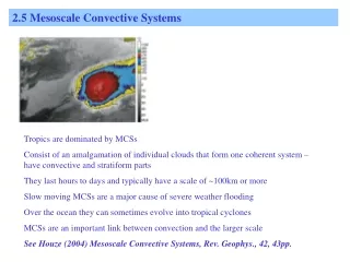
Motivation 1986 • Great Lakes region is an area of frequent MCS (MCC and derecho) activity • Important to understand behavior of MCSs when crossing the Great Lakes MCC Occurrences Frequency of Derechos Johns and Hirt (1987) Augustine and Howard (1991)
Areal Coverage ≥45 dBZ III II III I 0
Background 68% 8% 24% Graham et al. (2004)
Purpose • Present a climatology of MCSs that encountered Lake Michigan • Examine composite analyses of MCS environments associated with persisting and dissipating MCSs • Describe two MCSs, one that persisted and one that dissipated while crossing Lake Michigan and place them into context of the climatology and composites
MCS Selection Criteria • Warm Season (Apr–Sep) • 2002–2007 • MCSs in the study: • are ≥(100 50 km) on NOWrad composite reflectivity imagery • contain a continuous region ≥100 km of 45 dBZ echoes • meet the above two criteria for >3 h prior to crossing Lake Michigan 100 km 50 km
Climatology of MCSs n=110 • MCSs persisted upon crossing the lake if they: • continued to meet the two aforementioned reflectivity criteria • produced at least one severe report Dissipate Persist
Intersection Time after Formation n=110 Dissipate Persist
Monthly Distributions n=110 3.0°C 4.4°C 10.8°C 18.9°C 21.6°C 19.1°C Dissipate Persist
Hourly Distributions (UTC) n=110 Dissipate Persist
Synoptic-Scale Composites • Constructed using 0000, 0600, 1200, 1800 UTC 1° GFS analyses • Time chosen closest to intersection with Lake Michigan • If directly between two analysis times, earlier time chosen • Composited on MCS centroid and moved to the average position
Dynamic vs. Progressive Progressive Dynamic Johns (1993)
Dynamic Persist vs. Dissipate 200-hPa Heights (dam), 200-hPa Winds (m s-1), 850-hPa Winds (m s-1) n=17 n=31 m s−1 200-hPa m s−1 850-hPa Persist Dissipate
Dynamic Persist vs. Dissipate CAPE (J kg-1), 0–6 km Shear (barbs; m s-1) n=17 n=31 J kg−1 CAPE Persist Dissipate
Progressive Persist vs. Dissipate 200-hPa Heights (dam), 200-hPa Winds (m s-1), 850-hPa Winds (m s-1) n=30 n=32 m s−1 200-hPa m s−1 850-hPa Persist Dissipate
Progressive Persist vs. Dissipate CAPE (J kg-1), 0–6 km Shear (barbs; m s-1) n=30 n=30 n=32 n=32 J kg−1 CAPE Persist Dissipate
Case Studies 7–8 June 2008 - persist 4–5 June 2005 - dissipate
MCS 2105 UTC 7 June 08 - persist Source: UAlbany Archive 1600 UTC 4 June 05 - dissipate MCS Source: NOWrad Composites
2304 UTC 7 June 08 - persist MCS Source: UAlbany Archive 1800 UTC 4 June 05 - dissipate MCS Source: NOWrad Composites
0001 UTC 8 June 08 - persist MCS Source: UAlbany Archive 1900 UTC 4 June 05 - dissipate MCS Source: NOWrad Composites
0104 UTC 8 June 08 - persist MCS Source: UAlbany Archive 2000 UTC 4 June 05 - dissipate MCS Source: NOWrad Composites
0302 UTC 8 June 08 - persist MCS Source: UAlbany Archive 2200 UTC 4 June 05 - dissipate Source: NOWrad Composites
2000 UTC 7 June 08 - persist 26 23 26 23 29 20 29 32 04 26 08 MCS 16 18 12 32 Source: UAlbany Archive SLP (hPa), Surface Temperature (C), and Surface Mixing Ratio (>18 g kg-1)
1800 UTC 4 June 05 - dissipate 20 MCS 23 26 04 12 29 08 16 Source: UAlbany Archive SLP (hPa), Surface Temperature (C), and Surface Mixing Ratio (>16 g kg-1)
0000 UTC 8 June 08 - persist 2100 UTC 4 June 05 - dissipate 200-hPa Heights (dam), 200-hPa Winds (m s-1), 850-hPa Winds (barbs; m s-1) Source: 20-km RUC
0000 UTC 8 June 08 - persist 2100 UTC 4 June 05 - dissipate CAPE (J kg-1), 0–6 km Shear (barbs; m s-1) Source: 20-km RUC Source: 20-km RUC
4-h differences at 2300 UTC 7 June 08 - persist 975-hPa ∆(K), 0–3-km Shear (m s-1) ∆ (K), (K), Wind (m s-1) A 600 700 800 900 cold pool cold pool A’ A A’ A A 1900 UTC 2300 UTC Courtesy: M. Weisman Weisman and Rotunno (2004) A’ A’
4-h differences at 2300 UTC 7 June 08 - persist 975-hPa ∆(K), 0–3-km Shear (m s-1) A cold pool cold pool A’ A A’ A 2300 UTC 905 hPa
Madison, Wisconsin meteogram 975-hPa ∆ (K), 0–3 km Shear (m s-1) MSN Source: UAlbany Archive hPa °C T, Td, p
Buoy meteogram 975-hPa ∆ (K), 0–3 km Shear (m s-1) Buoy 45007 Source: NDBC °C hPa T=6.2°C Tair,Twater, p
2-h differences at 1900 UTC 4 June 05 - dissipate 975-hPa ∆(K), 0–3-km Shear (m s-1) ∆ (K), (K), Wind (m s-1) 600 700 800 900 B cold pool cold pool B’ B B’ B B B’ B’ 1900 UTC 1700 UTC
2-h differences at 1900 UTC 4 June 05 - dissipate 975-hPa ∆(K), 0–3-km Shear (m s-1) B cold pool cold pool B’ B B’ B 935 hPa
Aurora, Illinois meteogram 975-hPa ∆ (K), 0–3 km Shear (m s-1) Source: UAlbany Archive ARR hPa °C T, Td, p
Buoy meteogram 975-hPa ∆ (K), 0–3 km Shear (m s-1) °C hPa T=2.1°C Buoy 45007 Tair,Twater, p Source: NDBC
850-hPa Wind Climatology Differences Significant to 99.9th Percentile n=110 Persist Dissipate Source: NARR
Surface-Inversion Climatology Differences Significant to 95th Percentile T5m - TSfc Weak LLJ Later Season n=110 Persist Dissipate Source: NDBC
Phase Space - Warm Season Dissipate Persist All Months n=110 Source: NARR/NDBC
Dissipate Persist AMJ Phase Space - Early Season n=46 Dissipate Persist JAS Phase Space -Late Season n=64
Conclusions – Climatology • MCSs persisted 43% of the time (47 of 110 MCSs) upon crossing Lake Michigan during warm seasons of 2002–2007 • MCSs persisted and dissipated at a wide range of times after formation • MCSs persisted during all months and hours but favored July and August and evening and overnight • MCSs persisted with stronger 850-hPa winds and near-surface lake inversions, especially from April to July
Conclusions – Composites/Case Studies • Compared to MCSs that dissipated, MCSs persisted in environments that contained: • stronger 200-hPa and 850-hPa jet streams • larger amounts of CAPE and 0–6-km shear • similar looking synoptic-scale patterns • stronger, deeper convective cold pools • more stable marine layers