Download
1 / 69
1.66k likes | 4.39k Vues
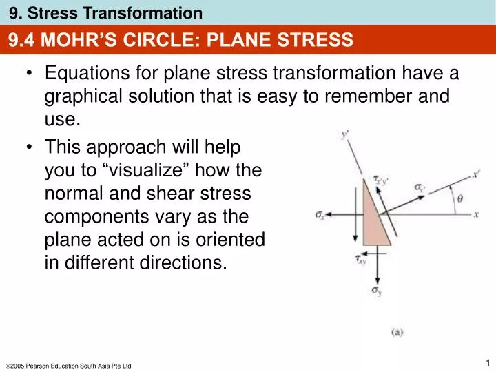
9.4 MOHR’S CIRCLE: PLANE STRESS . Equations for plane stress transformation have a graphical solution that is easy to remember and use. This approach will help you to “visualize” how the normal and shear stress components vary as the plane acted on is oriented in different directions.

E N D
9.4 MOHR’S CIRCLE: PLANE STRESS • Equations for plane stress transformation have a graphical solution that is easy to remember and use. • This approach will help you to “visualize” how the normal and shear stress components vary as the plane acted on is oriented in different directions.
9.4 MOHR’S CIRCLE: PLANE STRESS • Eqns 9-1 and 9-2 are rewritten as • Parameter can be eliminated by squaring each eqn and adding them together.
9.4 MOHR’S CIRCLE: PLANE STRESS • If x, y, xy are known constants, thus we compact the Eqn as,
9.4 MOHR’S CIRCLE: PLANE STRESS • Establish coordinate axes; positive to the right and positive downward, Eqn 9-11 represents a circle having radius R and center on the axis at pt C (avg, 0). This is called the Mohr’s Circle.
9.4 MOHR’S CIRCLE: PLANE STRESS • To draw the Mohr’s circle, we must establish the and axes. • Center of circle C (avg, 0) is plotted from the known stress components (x, y, xy). • We need to know at least one pt on the circle to get the radius of circle.
9.4 MOHR’S CIRCLE: PLANE STRESS Case 1 (x’ axis coincident with x axis) • = 0 • x’= x • x’y’ = xy. • Consider this as reference pt A, and plot its coordinates A (x, xy). • Apply Pythagoras theorem to shaded triangle to determine radius R. • Using pts C and A, the circle can now be drawn.
9.4 MOHR’S CIRCLE: PLANE STRESS Case 2 (x’ axis rotated 90 counterclockwise) • = 90 • x’= y • x’y’ = xy. • Its coordinates are G (y, xy). • Hence radial line CGis 180 counterclockwise from “reference line” CA.
9.4 MOHR’S CIRCLE: PLANE STRESS Procedure for Analysis Construction of the circle • Establish coordinate system where abscissa represents the normal stress , (+ve to the right), and the ordinate represents shear stress , (+ve downward). • Use positive sign convention for x, y, xy, plot the center of the circle C, located on the axis at a distance avg = (x + y)/2 from the origin.
9.4 MOHR’S CIRCLE: PLANE STRESS Procedure for Analysis Construction of the circle • Plot reference pt A (x, xy). This pt represents the normal and shear stress components on the element’s right-hand vertical face. Since x’ axis coincides with x axis, = 0.
9.4 MOHR’S CIRCLE: PLANE STRESS Procedure for Analysis Construction of the circle • Connect pt A with center C of the circle and determine CA by trigonometry. The distance represents the radius R of the circle. • Once R has been determined, sketch the circle.
9.4 MOHR’S CIRCLE: PLANE STRESS Procedure for Analysis Principal stress • Principal stresses 1 and 2 (1 2) are represented by two pts B and D where the circle intersects the -axis.
9.4 MOHR’S CIRCLE: PLANE STRESS Procedure for Analysis Principal stress • These stresses act on planes defined by angles p1 and p2. They are represented on the circle by angles 2p1 and 2p2and measured from radial reference line CA to lines CB and CD respectively.
9.4 MOHR’S CIRCLE: PLANE STRESS Procedure for Analysis Principal stress • Using trigonometry, only one of these angles needs to be calculated from the circle, since p1 and p2 are 90 apart. Remember that direction of rotation 2p on the circle represents the same direction of rotation p from reference axis (+x) to principal plane (+x’).
9.4 MOHR’S CIRCLE: PLANE STRESS Procedure for Analysis Maximum in-plane shear stress • The average normal stress and maximum in-plane shear stress components are determined from the circle as the coordinates of either pt Eor F.
9.4 MOHR’S CIRCLE: PLANE STRESS Procedure for Analysis Maximum in-plane shear stress • The angles s1 and s2 give the orientation of the planes that contain these components. The angle 2scan be determined using trigonometry. Here rotation is clockwise, and so s1 must be clockwise on the element.
9.4 MOHR’S CIRCLE: PLANE STRESS Procedure for Analysis Stresses on arbitrary plane • Normal and shear stress components x’ and x’y’acting on a specified plane defined by the angle , can be obtained from the circle by using trigonometry to determine the coordinates of pt P.
9.4 MOHR’S CIRCLE: PLANE STRESS Procedure for Analysis Stresses on arbitrary plane • To locate pt P, known angle for the plane (in this case counterclockwise) must be measured on the circle in the same direction 2(counterclockwise), from the radial reference line CA to the radial line CP.
EXAMPLE 9.9 Due to applied loading, element at pt A on solid cylinder as shown is subjected to the state of stress. Determine the principal stresses acting at this pt.
EXAMPLE 9.9 (SOLN) Construction of the circle • Center of the circle is at • Initial pt A (2, 6) and the center C (6, 0) are plotted as shown. The circle having a radius of
EXAMPLE 9.9 (SOLN) Principal stresses • Principal stresses indicated at pts B and D. For 1 > 2, • Obtain orientation of element by calculating counterclockwise angle 2p2, which defines the direction of p2 and 2 and its associated principal plane.
EXAMPLE 9.9 (SOLN) Principal stresses • The element is orientated such that x’ axis or 2 is directed 22.5 counterclockwise from the horizontal x-axis.
EXAMPLE 9.10 State of plane stress at a pt is shown on the element. Determine the maximum in-plane shear stresses and the orientation of the element upon which they act.
EXAMPLE 9.10 (SOLN) Construction of circle • Establish the , axes as shown below. Center of circle C located on the -axis, at the pt:
EXAMPLE 9.10 (SOLN) Construction of circle • Pt C and reference pt A (20, 60) are plotted. Apply Pythagoras theorem to shaded triangle to get circle’s radius CA,
EXAMPLE 9.10 (SOLN) Maximum in-plane shear stress • Maximum in-plane shear stress and average normal stress are identified by pt E or F on the circle. In particular, coordinates of pt E (35, 81.4) gives
EXAMPLE 9.10 (SOLN) Maximum in-plane shear stress • Counterclockwise angle s1 can be found from the circle, identified as 2s1.
EXAMPLE 9.10 (SOLN) Maximum in-plane shear stress • This counterclockwise angle defines the direction of the x’ axis. Since pt E has positive coordinates, then the average normal stress and maximum in-plane shear stress both act in the positive x’ and y’ directions as shown.
EXAMPLE 9.11 State of plane stress at a pt is shown on the element. Represent this state of stress on an element oriented 30 counterclockwise from position shown.
EXAMPLE 9.11 (SOLN) Construction of circle • Establish the , axes as shown. Center of circle Clocated on the -axis, at the pt:
EXAMPLE 9.11 (SOLN) Construction of circle • Initial pt for = 0 has coordinates A (8, 6) are plotted. Apply Pythagoras theorem to shaded triangle to get circle’s radius CA,
EXAMPLE 9.11 (SOLN) Stresses on 30 element • Since element is rotated 30 counterclockwise, we must construct a radial line CP, 2(30) = 60 counterclockwise, measured from CA ( = 0). • Coordinates of pt P (x’, x’y’) must be obtained. From geometry of circle,
EXAMPLE 9.11 (SOLN) Stresses on 30 element • The two stress components act on face BD of element shown, since the x’ axis for this face if oriented 30 counterclockwise from the x-axis. • Stress components acting on adjacent face DE of element, which is 60 clockwise from +x-axis, are represented by the coordinates of pt Q on the circle. • This pt lies on the radial line CQ, which is 180 from CP.
EXAMPLE 9.11 (SOLN) Stresses on 30 element • The coordinates of pt Q are • Note that here x’y’ acts in the y’ direction.
9.5 STRESS IN SHAFTS DUE TO AXIAL LOAD AND TORSION • Occasionally, circular shafts are subjected to combined effects of both an axial load and torsion. • Provided materials remain linear elastic, and subjected to small deformations, we use principle of superposition to obtain resultant stress in shaft due to both loadings. • Principal stress can be determined using either stress transformation equations or Mohr’s circle.
EXAMPLE 9.12 Axial force of 900 N and torque of 2.50 Nm are applied to shaft. If shaft has a diameter of 40 mm, determine the principal stresses at a pt P on its surface.
EXAMPLE 9.12 (SOLN) Internal loadings • Consist of torque of 2.50 Nm and axial load of 900 N. Stress components • Stresses produced at pt P are therefore
EXAMPLE 9.12 (SOLN) Principal stresses • Using Mohr’s circle, center of circle Cat the pt is • Plotting C (358.1, 0) and reference pt A (0, 198.9), the radius found was R = 409.7 kPA. Principal stresses represented by pts B and D.
EXAMPLE 9.12 (SOLN) Principal stresses • Clockwise angle 2p2 can be determined from the circle. It is 2p2 = 29.1. The element is oriented such that the x’ axis or 2 is directed clockwise p1 = 14.5 with the x axis as shown.
9.6 STRESS VARIATIONS THROUGHOUT A PRISMATIC BEAM • The shear and flexure formulas are applied to a cantilevered beam that has a rectangular x-section and supports a load P at its end. • At arbitrary section a-a along beam’s axis, internal shear Vand moment M are developed from a parabolic shear-stress distribution, and a linear normal-stress distribution.
9.6 STRESS VARIATIONS THROUGHOUT A PRISMATIC BEAM • The stresses acting on elements at pts 1 through 5 along the section. • In each case, the state of stress can be transformed into principal stresses, using either stress-transformation equations or Mohr’s circle. • Maximum tensile stress acting on vertical faces of element 1 becomes smaller on corresponding faces of successive elements, until it’s zero on element 5.
9.6 STRESS VARIATIONS THROUGHOUT A PRISMATIC BEAM • Similarly, maximum compressive stress of vertical faces of element 5 reduces to zero on that of element 1. • By extending this analysis to many vertical sections along the beam, a profile of the results can be represented by curves called stress trajectories. • Each curve indicate the direction of a principal stress having a constant magnitude.
EXAMPLE 9.13 Beam is subjected to the distributed loading of = 120kN/m. Determine the principal stresses in the beam at pt P, which lies at the top of the web. Neglect the size of the fillets and stress concentrations at this pt. I = 67.1(10-6) m4.
EXAMPLE 9.13 (SOLN) Internal loadings • Support reaction on the beam B is determined, and equilibrium of sectioned beam yields Stress components • At pt P,
EXAMPLE 9.13 (SOLN) Stress components • At pt P, Principal stresses • Using Mohr’s circle, the principal stresses at P can be determined.
EXAMPLE 9.13 (SOLN) Principal stresses • As shown, the center of the circle is at (45.4 + 0)/2 = 22.7, and pt A (45.4, 35.2). We find that radius R = 41.9, therefore • The counterclockwise angle 2p2 = 57.2, so that
9.7 ABSOLUTE MAXIMUM SHEAR STRESS • A pt in a body subjected to a general 3-D state of stress will have a normal stress and 2 shear-stress components acting on each of its faces. • We can develop stress-transformation equations to determine the normal and shear stress components acting on ANY skewed plane of the element.
9.7 ABSOLUTE MAXIMUM SHEAR STRESS • These principal stresses are assumed to have maximum, intermediate and minimum intensity: max int min. • Assume that orientation of the element and principal stress are known, thus we have a condition known as triaxial stress.
9.7 ABSOLUTE MAXIMUM SHEAR STRESS • Viewing the element in 2D (y’-z’, x’-z’,x’-y’) we then use Mohr’s circle to determine the maximum in-plane shear stress for each case.
9.7 ABSOLUTE MAXIMUM SHEAR STRESS • As shown, the element have a45 orientation and is subjected to maximum in-plane shear and average normal stress components.
9.7 ABSOLUTE MAXIMUM SHEAR STRESS • Comparing the 3 circles, we see that the absolute maximum shear stress is defined by the circle having the largest radius. • This condition can also be determined directly by choosing the maximum and minimum principal stresses: