Download
1 / 21
210 likes | 378 Vues
NSTX. Supported by. Investigation of microtearing modes for electron transport in NSTX. College W&M Colorado Sch Mines Columbia U CompX General Atomics INEL Johns Hopkins U LANL LLNL Lodestar MIT Nova Photonics New York U Old Dominion U ORNL PPPL PSI Princeton U Purdue U SNL

E N D
NSTX Supported by Investigation of microtearing modes for electron transport in NSTX College W&M Colorado Sch Mines Columbia U CompX General Atomics INEL Johns Hopkins U LANL LLNL Lodestar MIT Nova Photonics New York U Old Dominion U ORNL PPPL PSI Princeton U Purdue U SNL Think Tank, Inc. UC Davis UC Irvine UCLA UCSD U Colorado U Illinois U Maryland U Rochester U Washington U Wisconsin Culham Sci Ctr U St. Andrews York U Chubu U Fukui U Hiroshima U Hyogo U Kyoto U Kyushu U Kyushu Tokai U NIFS Niigata U U Tokyo JAEA Hebrew U Ioffe Inst RRC Kurchatov Inst TRINITI KBSI KAIST POSTECH ASIPP ENEA, Frascati CEA, Cadarache IPP, Jülich IPP, Garching ASCR, Czech Rep U Quebec Presented by King-Lap Wong Co-authors: D. Mikkelsen, J. Krommes, K. Tritz, D.R. Smith, S. Kaye ITPA Meeting PPPL Oct. 5-7, 2009
Outline • Introduction • Properties of microtearing modes • Proposed experiment on NSTX • Some ideas for AUG • Summary
Introduction Anomalous edue to imperfect magnetic surfaces: • Magnetic islands - Kerst 1962, Rosenbluth, Sadeev, Taylor 1966 • Magnetic braiding - Stix 1973 • e in stochastic magnetic field - R & R 1978, Stix 1978 • Lc~ qR for tokamak - Kadomtsev 1978, Krommes 1983 • properties of microtearing - Drake, Gladd, D’Ippolito, Connor 1980 -1990 • In conventional tokamaks, microtearing can only be found at the edge (D-III 1987, CMOD 1999) • In STs, microtearing can be the dominant instability - Redi 2003, Applegate 2004 • Microtearing can explain measured e at r/a>0.5 in NSTX, Wong - 2007 • Microtearing can be unstable at the outer core of AUG, Told - 2008 Can we find experimental evidence of this instability ?
Properties of microtearing modes • High-m (m~10-20) tearing modes (k||=0) • Driven mainly by Te ’ is actually negative at high m (stabilizing) Different from ITG modes : • ErBr||mode structurek direction Microtearing odd even extended electron drift • ITG even odd ballooning ion drift Br has even parity - creates magnetic islands at q=m/n • In slab geometry, microtearing instability requires: [Wesson, “Tokamaks”, 1987] (a) e= dlnTe/dlnne > 0.3 (b) collision rate must exceed electron diamagnetic freq., ei > ★e
Distinguishing between microtearing and resistive ballooning modes • Frequency microtearing: = ★e + c ★T , 0 < c < 1 resistive ballooning: << ★e • Mode structure microtearing:k|| = 0 mode structure extended along B resistive ballooning: k||≠ 0, mode amplitude peaks on low field side, because the bad curvature plays an important role
Growth rate of microtearing modes (NSTX#116313, 0.9s) many unstable modes broadband spectrum expected
K-L Wong, APS-07, NI1.00004, p 7 Comparison between etheoryandeexp Put B/B=e/LT, get e = (e/LT)2 Rve(mfp/Lc)= (e/LT)2ve2/(eiq) Use parameters from #116313A11 at 0.9s, Lc= qR
K-L Wong, APS-07, NI1.00004, p 8 Microtearing modes are stable at low ei (< ★e ) Reduce transport by lowering ne and raising Te
Scaling of tE with ei in NSTX • In beam heated plasmas, Te(0) < 1 keV, ne(0) < 1014 cm-3 • In HHFW heated plasmas, Te(0) < 5 keV, ne(0) < 3x1013 cm-3 • NSTX data base appear to support microtearing mode as the dominant cause of electron heat loss in many beam heated plasmas – see K. Tritz’s presentation
Transition to global stochasticitymany possibilities, but they are not equally probable • Landau-Hopf scenario - the power spectrum should have finite discrete frequencies (finite no. modes) - not observed in experiment highly unlikely • Ruelle-Takens scenario - broadband noise (chaos) appear in power spectrum after a few bifurcations likely to be the case • Don’t expect to see linear growth of a coherent single mode prepare to deal with stochastic magnetic field over an extended region (fully developed magnetic turbulence) • Lesson learned from TEM/ITG: need to work with plasma in stochastic B.
Mirnov loop lacks spatial resolution- not too useful for broadband high m,n fluctuations deep inside the plasma
Work with the tools we have: the X-ray camera Ref: Stutman et al., RSI 74,1982 (2003)
X-ray emissivity • For Maxwellian electrons in NSTX plasmas, X-ray emission is dominated by collisional excitation of impurity ions1; dielectronic recombination2 is small; bremsstrahlung3(ff) and radiative recombination4 (fb) are very small • Emissivity for both (1), (2) & (3) scale like ~ ne nz (Z e)2 √Te • is approximately constant on a flux surface for NSTX plasmas - see Stutman et al., RSI 74,1982 (2003) • Te & ne fluctuations - Te & dnegive rise to which may be measurable in NSTX
Crude estimates • Take parameters from #116313, r/a=0.5, t=0.9s • Island full width: ∆r = 4 ( bmn R r q / m s )1/2 ~ 0.85 cm • Put r ≤ ∆r / 2 ~ 0.4 cm, Ln ~ 50 cm, LT ~ 35 cm, • get ~ r / Ln + 0.5 r / LT ~ 1.4% • ~ 1% is not too difficult to detect if we have a diagnostic that can do localmeasurements • However, all we have is an X-ray camera for line-of-sight measurements - difficult !
SVD analysis • Ref: T. Dudok de Wit et al., PoP 1, 3228(1994) • Expand the discrete signal (n x m matrix) y(xj, ti) into a set of modes that are orthogonal in time and space y(xj, ti) = k=1 KAkk(xj) k(ti), K = min(n,m) • Chrono = temporal eigenfunction = k(ti) • Topo = spatial eigenfunction = k(xj) • Weight distribution: Ak (≥0), k =1, 2, ….. K • Construct the matrix Yi j = y(xj, ti) and use IDL subroutine to do SVD analysis - program written by David Smith
Preliminary SVD results (15 Ch SXR) • Topo frequently exhibits wave-packet structure although the camera spatial resolution is marginal • Chrono usually consists of irregular / intermittent bursts • No sign of single mode growth - has temporal resolution - fNyquist= 300kHz , i.e., Landau’s Scenario NOT observed • No single frequency signal observed - usually see broadband fully developed turbulence (Ruelle-Takens scenario ?) • A lot more data / work are needed
Need data from all 46 channels • Need to do cross correlations of ij(xij) for xij on same flux surface • New software capabilities (new tools) needed: Overlay plots of flux surfaces (from EFIT or TRANSP) and X-ray viewing chords Search for coherent structures, correlation lengths etc, Don’t expect quick success from this experiment - need to stop & think every step along the way
De and the X-ray energy spectrum • Kinetic eq: ∂f/∂t = e/m E∂f/∂v + C(f) + LDeLf L = ∂/∂x - (eEA/m)/v2 E - applied electric field(1st order), EA - ambipolar electric field • Perturbative solution: f = f(0) + f(1) + f(2) + …. • 0-th order: 0 = C(f(0)) local Maxwellian • 1st order: 0 = C(f(1)) - e/m E ∂f(0)/∂v Spitzer resistivity • 2nd order: 0 = C(f(2)) + LDeLf(0) - e/m E ∂f(1)/∂v and f(2) gives information on De • Ref: K. Molvig et al., PRL 41, 1240 (1978) – formulation looks fine, result is questionable First step: Use X-ray spectrometer to look for non-Maxwellian fe(v) 2nd step: Measure f(r,v,t) with PILATUS detector modules and solve for De
Some ideas for AUG – more hardware capability • Heat pulse propagation expt with ECH & ECE for Te(r,t) - directly determine e. • Use fast electrons from ECH at high_B side as trace particles and measure spatial diffusion of trace particles due to stochastic B – DM ? • Measure f(r,v,t) with PILATUS detector modules and solve for De • Tangential viewing port will be helpful if Ee~100keV Cross-polarization scattering to measure B ?
Summary • Identification of a single microtearing mode in linear growth phase is difficult – not expected based on current knowledge: Can MSE and / or JHU’s technique work? - Probably not, but … Never hurt to try. • Need to prepare for fully developed turbulence – plasma in stochastic magnetic fieldNeed theoretical input: Do we know how to describe the plasma equilibrium ? Ref: Reiman et al., Nucl.Fusion(2007); Krommes et al., J. Plasma Physics (1983). • For ST’s (NSTX / MAST): X-ray spectrometer may provide some evidence of non-Maxwellian fe(v) Multi-chord imaging can provide more info’ – PILATUS has the best chance • For AUG: ECH + ECE provides new capabilities not available on STs PILATUS with tangential view possible? • PPPL owns two PILATUS (now on CMOD), asking for a 3rd one Are they available for collaborative microtearing expts ?