Download
1 / 27
270 likes | 516 Vues
Pendulum Modeling in Mathematica ™ and Matlab ™. IGR Thermal Noise Group Meeting 4 May 2007. The X-Pendulum. Developed as a low frequency vibration isolator for TAMA. 1D version. 2D version. Pendulum Modelling.

E N D
Pendulum Modeling in Mathematica™ and Matlab™ IGR Thermal Noise Group Meeting 4 May 2007
The X-Pendulum • Developed as a low frequency vibration isolator for TAMA 1D version 2D version
Pendulum Modelling • Wanted an AdvLIGO SUS design model to go beyond the Matlab model of Torrie, Strain et al. • Desired features: • Full 3D with provision for asymmetries • Proper blade model • Wire bending elasticity • Arbitrary damping and consequent thermal noise • Export to other environments such as Matlab/Simulink and E2E. • Mathematica code originally developed for modeling the X-pendulum was available -> reuse and extend. • See http://www.ligo.caltech.edu/~e2e/SUSmodels • Manual: T020205-00 (-01 pending)
The Toolkit • The toolkit is a Mathematica “package”, PendUtil.nb, for specifying different configurations (e.g., quad, triple etc) in a (relatively) user-friendly way • Supported features: • 6-DOF rigid bodies for masses (no internal modes) • Springs described by an elasticity tensor and a vector of pre-load forces • Massless wires (i.e., no violin modes) but detailed elasticity model from beam equation • Arbitrary frequency-dependent damping on all sources of elasticity • Symbolic up to the point of minimizing the potential to find the equilibrium position • Calculates elasticity and mass matrices semi-numerically (symbolic partial derivatives of functions with mostly numeric coefficients) • Eigenfrequencies and eigenmodes calculated numerically • Arbitrary frequency dependent damping on each different elastic element • Transfer functions • Thermal noise plots • Export of state-space matrices to Matlab and E2E
Models • Two major families of models have been defined: • The triple models reflect a generic GEO-style pendulum with 3 masses, 6 blade springs and 10 wires. • The quad models reflect a standard AdvLIGO quad pendulum, with 4 masses, 6 blade springs and 14 wires. • Many toy models • LIGO-I two-wire pendulum • Simple pendulum • Simple pendulum on a blade spring • Etc • Steep learning curve but a major new model can be programmed in a day by an experienced user 5
Triple Pendulum Model • 2 blade springs • 2 wires • “upper” mass • 4 blade springs • 4 wires • “intermediate” mass • 4 fibres • optic 6
Quad Pendulum • 2 blade springs • 2 wires • “top” mass • 2 blade springs • 4 wires • “upper” mass • 2 blade springs • 4 wires • “intermediate” mass • 4 fibres • optic 7
Defining a Model (i) • Define the “variables” (cf. x in the theory - example from the xtra-lite triple): • allvars = { • x1,y1,z1,yaw1,pitch1,roll1, • x2,y2,z2,yaw2,pitch2,roll2, • x3,y3,z3,yaw3,pitch3,roll3 • }; • Define the “floats” (cf. q in the theory): • allfloats = { • qul,qur,qlf,qlb,qrf,qrb • }; • Define the “parameters” (cf. s in the theory): • allparams = { • x00, y00, z00, yaw00, pitch00, roll00 • }; 8
Defining a Model (ii) • Define coordinate lists for rigid bodies of interest: • optic = {x3, y3, z3, yaw3, pitch3, roll3}; • support = {x00, y00, z00, yaw00, pitch00, roll00}; • Define coordinate lists for points on rigid bodies • massUl={0,-n1,d0}; (* left wire attachment point on upper mass *) • Define list of gravitational potential terms: • gravlist = {}; (* initialize list *) • AppendTo[gravlist, m3 g z3]; (* typical item *) 9
Defining a Model (iii) • Define list of wires, each with the following format • { • coordinate list defining first mass, • attachment point for first mass (local coordinates), • attachment vector for first mass, • coordinate list defining second mass, • attachment point for second mass (local coordinates), • attachment vector for second mass, • Young's modulus, • unstretched length, • longitudinal elasticity, • vector defining principal axis 1, • moment of area along principal axis 1, • moment of area along principal axis 2, • linear elasticity type, • angular elasticity type, • torsional elasticity type, • shear modulus, • cross sectional area for torsional calculations, • torsional stiffness geometric factor • } 10
Defining a Model (iv) • Define list of springs, each with following format: • { • coordinate list defining first mass, • attachment point for first mass (local coordinates), • attachment angles for first mass (yaw, pitch, roll), • coordinate list defining second mass, • attachment point for second mass (local coordinates), • attachment angles for second mass (yaw, pitch, roll), • damping type, • 6x6 elasticity matrix, • 1*6 pre-load force/torque vector • } • Define kinetic energy • IM3 = {{I3x, 0, 0}, {0, I3y, 0}, {0, 0, I3z}}; (* typical MOI tensor) • kinetic = ( • … • +(1/2) m3 Plus@@(Dt[b2s[optic,COM],t]^2) • +(1/2) omegaB[yaw3, pitch3, roll3].IM3.omegaB[yaw3, pitch3, roll3] • … • ); 11
Defining a Model (v) • Define default values of constants • defaultvalues = { • g -> 9.81, (* value given numerically *) • … • m3 -> Pi*r3^2*t3, (* value given in terms of other constants *) • … • x00 -> 0, (* value for nominal position of structure *) • y00 -> 0, • z00 -> 0, • … • damping[imag,dampingtype] -> (phi&) (* value for frequency dependence of damping *) • … • }; • Define starting point for finding equilibrium position: • startpos = { • x1 ->0, • y1 ->0, • … • }; 12
Defining a Model (vi) • Define model-specific utilities: • A function to list eigenmodes in a table • pretty[eigenvector] • A function to plot eigenmode shapes • eigenplot[eigenvector, amplitude, {viewpoint}] • Vectors representing force and displacement inputs and displacement outputs of interest • structurerollinput = makeinputvector[roll00]; • opticxinput = makefinputvector[x3]; • opticx = makeoutputvector[x3]; • Rotation matrices to put angle variables in a more easily interpretable basis: • e2ni; 13
Sample Output (i) • Transfer function from x displacement of support to x motion of optic (quad model, reference parameters of 20031114):
Damping • Damping can be represented by a complex elastic modulus: • Strictly, the Kramers-Kronig relation applies: • However often the variation in the real part can be ignored: • Need to consider total potential as sum of terms, each with different damping: 15
Sample Output (ii) • Thermal noise in x motion of optic (quad model, reference parameters of 20031114):
Application to Quad Controls • Good agreement after adding lots of new physics: • Improved wire flexure correction • Blade lateral compliance • Blade geometric antispring effect • Non-diagonal moment of inertia tensors ID pitch x y z yaw roll x y pitch yaw x y z yaw pitch roll yaw pitch? roll x z roll z roll f (theory) 0.395 0.443 0.464 0.595 0.685 0.810 0.987 1.043 1.167 1.428 1.981 2.095 2.362 2.538 2.818 2.762 3.167 3.228 3.332 3.401 3.793 5.120 17.700 25.741 f (exp) 0.403 0.440 0.464 0.549 0.684 0.794 0.989 1.038 1.355 1.428 1.978 2.075 2.222 2.515 2.576 2.734 3.149 3.162 3.333 3.381 3.589 5.029 ? ?
Dissipation Dilution • Often said: main restoring force in a pendulum is gravitational therefore no loss -> “dissipation dilution” • Not true! • Gravitational force is purely vertical. • Actual restoring force is sideways component of tension in wire • Gravity’s only contribution is to tension the wire. • Other forms of tension are equivalent (cf. violin modes also low-loss • What is it about tension? 20
Non-dilution case (vertical) • Mass on spring • Force: • Frequency: • Amplitude (phasor): • Velocity (phasor): • Force (phasor): • Power (average): • Energy (max): • Decay time (energy): • Decay time (amp.) 21
Dilution case (horizontal - exactly) • Constrain mass to move exactly horizontally • Restoring force: • Spring constant: • Frequency: • Length: • Power: • Energy: • Energy still 2nd order but power 4th order
But what about pendulums?! • In a pendulum, mass really moves on an arc. • Doesn’t matter! • Normal mode analysis can’t tell the difference! • Eigenmodes are always linear in coordinates used. • Analyze in r,theta -> eigenmode is arc • Analyze in x, z -> eigenmode is straight line • Same frequencies!
What about pendulums (ii) • Two independent reasons why pendulums have low loss. • Restoring force is sideways component of tension • Energy may then be off-loaded into gravitational potential -> stretch of spring less even than second order • Depends on bounce and pendulum mode frequencies • Usual case, bounce frequency high -> mass moves on arc. • Very low bounce frequencies (superspring) -> mass really does move horizontally 24
Dissipation Dilution and Mathematica Toolkit • Solution used in toolkit: • Keep a separate stiffness matrix Pi for each elastic element • For all elasticity types that depend on tension • Compute potential matrix once normally • Recompute with tension zeroed out. • Apply damping to stiffness components that persist with tension off • Need to do analogous thing for ANSYS • Difficult because detailed potential data not available, or at least not easy to access. 25
Test Case for ANSYS: Violin modes of a fibre • Fibre under tension behaves as if shortened by flexure correction at each end • Energy of two types • Longitudinal stretching from bending out of straight line (low-loss) • Bending energy (lossy) Sinusoid End correction Total
Fibre results • Fused silica, 350 mm long, 0.45 mm diameter • Integrand of the two types • Longitudinal -> • Total 17.3 mJ for 10 mm amplitude • Bending -> • Total 0.256 mJ for 10 mm amplitude • Dissipation dilution factor 67.6 • Will compare to ANSYS