Download
1 / 37
370 likes | 381 Vues
Inventory Optimization under Correlated Uncertainty. Abhilasha Aswal G N S Prasanna, International Institute of Information Technology – Bangalore. Outline. Motivation Optimizing with correlated demands Generalized EOQ Related work Some Extensions: Generalized base stock Geman Tank

E N D
Inventory Optimization under Correlated Uncertainty Abhilasha Aswal G N S Prasanna, International Institute of Information Technology – Bangalore
Outline • Motivation • Optimizing with correlated demands • Generalized EOQ • Related work • Some Extensions: • Generalized base stock • Geman Tank • Relational Algebra • Conclusions
Q* The EOQ model • The EOQ model (Classical – Harris 1913) • C: fixed ordering cost per order • h: per unit holding cost • D: demand rate • Q*: optimal order quantity • f*: optimal order frequency
Car type I Car type II Car type III Automobile store Tyre type I Supplies Tyre type II Petrol Drivers Motivation • Inventory optimization example
Motivation • Ordering and holding costs
1 product versus 7 products • Exactly Known Demands, no uncertainty • EOQ solution and Constrained Optimization solution match exactly: • But… UNREALISTIC!!! We cannot know the future demands exactly.
1 product versus 7 products • Bounded Uncorrelated Uncertainty • Assuming the range of variation of the demands is known, we can get bounds on the performance by optimizing for both the min value and the max value of the demands. • EOQ solution and Constrained Optimization solution are almost the same.
1 product versus 7 products • Beyond EOQ: Correlated Uncertainty in Demand • Considering the substitutive effects between a class of products (cars, tyres etc.) 200 ≤ dem_tyre_1 + dem_tyre_2 ≤ 700 65 ≤ dem_car_1 + dem_car_2 + dem_car_3 ≤ 250 • Considering the complementary effects between products that track each other 5 ≤ (dem_car_1 + dem_car_2 + dem_car_3) – dem_petrol ≤ 20 5 ≤ dem_car_2 – dem_drivers ≤ 20 EOQ cannot incorporate such forms of uncertainty.
1 product versus 7 products • Beyond EOQ: Correlated Uncertainty in Demand • Min-Max solution for different scenarios:
1 product versus 7 products • Beyond EOQ: Correlated Uncertainty in Demand • Comparison of different uncertainty sets
Optimizing with Correlated DemandsMathematical Programming Formalism
Optimal Inventory policy using “ILP” • Min-max optimization, not an LP. • Duality?? • Fixed costs and breakpoints: non-convexities that preclude strong-duality from being achieved. • No breakpoints or fixed costs: min-max optimization QP • Heuristics have to be used in general.
Optimal Inventory policy by Sampling • A simple statistical sampling heuristic Begin for i = 1 to maxIteration { parameterSample = getParameterSample(constraint Set) bestPolicy = getBestPolicy(parameterSample) findCostBounds(bestPolicy) } chooseBestSolution() End
Optimizing with Correlated Demands:Analytical Formulation: Generalized EOQ(K)
Classical EOQ model • Per order fixed cost = f(Q) • holding cost per unit time = h(Q)
EOQ(K) with multiple products, uncertain demands • Additive SKU costs Case with 2 commodities, generalized to ncommodities
EOQ(K) with multiple products, uncertain demands • Holding cost linear, ordering cost fixed
Analytical solution: Substitutive constraints • Holding cost linear, ordering cost fixed • Under a substitutive constraint D1 + D2 <= D
Analytical solution: Substitutive constraints - Example • 2 products, demands D1 & D2 • Costs: h1 = 2/unit h2 = 3/unit f1 = 5/order f2 = 5/order • D1 + D2 = D = 100 • Maximum cost • Minimum cost
Analytical solution: Complementary constraints • Holding cost linear, ordering cost fixed • Under a complementary constraint D1 – D2 <= D, with D1 and D2 limited to Dmax
Analytical solution: Complementary constraints - Example • 2 products, demands D1 & D2 • Costs: h1 = 2/unit h2 = 3/unit f1 = 5/order f2 = 5/order • Demand constraints: D1 - D2 = K = 20 D1 <= Dmax = 50 D2 <= Dmax = 50 • Maximum cost • Minimum cost
Both substitutive & complementary constraints • Holding cost linear, ordering cost fixed • Under both substitutive and complementary constraints • Convex optimization techniques are required for this optimization.
Both substitutive & complementary constraints - Optimization • Objective function: concave • Minimization: HARD! • Envelope based bounding schemes • Heuristics to find upper bound. • Simulated annealing based
Both substitutive & complementary constraints - Example • 2 products, demands D1 & D2 • Costs: h1 = 2/unit h2 = 3/unit f1 = 5/order f2 = 5/order • Demand constraints: 150 <= D1 + D2 <= 200 -20 <= D1 – D2 <= 20 • Maximum cost: 99.88 • Minimum cost • Enumerating all vertices (exact) 85.39 • Simulated annealing heuristic 85.48499 • Error: 0.111247 %
Both substitutive & complementary constraints – Example (contd) • 5 products, demands D1, D2, D3, D4 & D5 • Costs: h1 = 2/unit h2 = 3/unit h3 = 4/unit h4 = 5/unit h5 = 6/unit f1, f2, f3, f4, f5 = 5/order • Demandconstraints: D1 + D2 + D3 + D4 + D5 <= 1000 D1 + D2 + D3 + D4 + D5 >= 500 2 D1 - D2 <= 400 2 D1 - D2 >= 100 5 D5 - 2 D4 <= 900 5 D5 - 2 D4 >= 150 D2 + D4 <= 400 D2 + D4 >= 250 D1 <= 350 D1 >= 100 D3 >= 150 D3 <= 300 D4 >= 75 D4 <= 200
Both substitutive & complementary constraints – Example (contd) • Maximum cost: 436.6448 • Minimum cost: • Enumerating all vertices (exact) 323.5942 • Simulated annealing heuristic 324.4728 • Error: 0.271505 %
Inventory constraints • Constrained Inventory Levels • If the inventory levels Qi and demands Di, are constrained as • The vector constraint above can incorporate constraints like • Limits on total inventory capacity (Q1+Q2 <= Qtot) • Balanced inventories across SKUs (Q1-Q2) <= ∆ • Inventories tracking demand (Q1-D1<=Dmax)
Inventory constraints • Constrained Inventory Levels
Related Work • McGill (1995) • Inderfurth (1995) • Dong & Lee (2003) • Stefanescu et. al. (2004) • Bertsimas, Sim, Thiele et. al.
Related work • Bertsimas, Sim, Thiele - “Budget of uncertainty” • Uncertainty: • Normalized deviation for a parameter: • Sum of all normalized deviations limited: • N uncertain parameters polytope with 2N sides • In contrast, our polyhedral uncertainty sets: • More general • Much fewer sides
The German Tank Problem Classical German Tank Generalization Given correlated data samples, drawn from a uniform distribution- estimating the bounded region formed by correlated constraints enclosing the samples. Estimating the constraints without bias and with minimum variance. • Biased estimators • Maximum likelihood • Unbiased estimators • Minimum Variance unbiased estimator (UMVU) • Maximum Spacing estimator • Bias-corrected maximum likelihood estimator
Information Theory and Relational Algebra • Uncertainty can be identified with Information. • Information polyhedral volume • Relational algebra between alternative constraint polyhedra
Conclusions • Generalized EOQ to Correlated Demands • Analytical Solutions • Computational Solutions • Enumerative versus Simulated Annealing • Extensions of formulations • Generalized Basestock • German Tank • Information Theory and Relational Algebra