Download
1 / 14
150 likes | 321 Vues
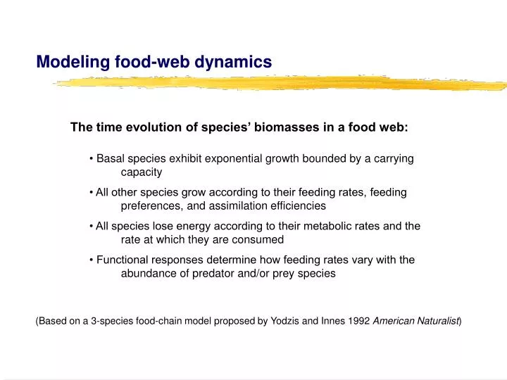
Modeling food-web dynamics. The time evolution of species’ biomasses in a food web: • Basal species exhibit exponential growth bounded by a carrying capacity • All other species grow according to their feeding rates, feeding preferences, and assimilation efficiencies

E N D
Modeling food-web dynamics The time evolution of species’ biomasses in a food web: • Basal species exhibit exponential growth bounded by a carrying capacity • All other species grow according to their feeding rates, feeding preferences, and assimilation efficiencies • All species lose energy according to their metabolic rates and the rate at which they are consumed • Functional responses determine how feeding rates vary with the abundance of predator and/or prey species (Based on a 3-species food-chain model proposed by Yodzis and Innes 1992 American Naturalist)
n ( ) å Bi’(t) = Gi(B) – xi Bi (t) + xi yijαij Fij (B) Bi (t) – xj yjiαji Fji (B) Bj (t) / eji j =1 Rate of change = Production rate – Loss of biomass + Gain of biomass – Loss of biomass to in biomass if species i is basal to metabolism from resource spp. consumer spp. Nonlinear bioenergetic ecosystem model The variation of Bi, the biomass of species i, is given by: What factors allow persistence of species in dynamical models of complex food webs? (the “devious strategies”)
G ( B ) i 3 species parameters: : production rate of basal speciesi(Mass/Time) For primary producers, Gi (B) = ri Bi (t) (1 – Bi (t) / K i ), where ri : intrinsic growth rate of species i(1/Time) Ki : carrying capacity of species i(Mass) ______________ xi : mass-specific metabolic rate of species i(Mass/Time * 1/Mass) 4 species interaction parameters: eji : assimilation efficiency of species j consuming species i(fraction of biomass) yij : rate of maximum biomass gain by species i consuming j normalized by metabolic rate of species i (Mass/Time / Mass/Time) αij : relative preference of species ifor species j(fraction of diet) (αij= 0 for producers and sums to 1 for consumers) Fij (B) : non-dimensional functional response (based on parameters q or c) (relative consumption rate of predator species i consuming prey species j as a fraction of the maximum ingestion rate; function of species’ biomass)
Parameterized Functional responses Type II (dominates nonlinear population dynamics modeling; q or c = 0) - ƒ(prey density) - function of predator search and prey handling times Type III (q = 1) - ƒ(prey density) - predation on low-density prey relaxed; successful food searches increases predator’s search effort Predator Interference (c = 1) - ƒ(prey & predator densities) - increase in predators decreases predation due to interference among predators - matches empirical data much better than Type II (Skalski & Gilliam 2001)
q = 1 c = 0 c = 1 B ( t ) Addition of Predator Interference to Type II Functional Response: j = F ( ) B ij n å a + + B ( t ) ( 1 c B ( t )) B ik k ij i 0 ji = k 1
3-species dynamics & functional response Slight increases in Predator Interference or Type III stabilize dynamics chaotic dynamics period doubling reversals stabilization of limit cycles stable stationary solution Type III Predator Interference biomass local min/max (top predator) local min & max functional response parameters When c or q = 0, the functional response is Type II
biomass min & max 10-species dynamics & functional response Strong Type II FR may stress dynamics by increasing feeding on rarer species while decreasing it on more abundant species. At q = 0 (conventional strong Type II response), only 4 taxa display persistent dynamics. At q > 0.15 (very weak Type III response), all 10 taxa are persistent. At q > 0.3 (weak Type III response), all 10 taxa are steady-state. functional response
Holling Type II / III 0.7 0.6 0.5 0.4 Robustness 0.3 0.2 0.1 0 0 0.05 0.1 0.15 0.2 0.25 0.3 q Stabilization of Dynamics of Ecological Networks (S=30, C=0.15) with Functional Responses Beddington-DeAngelis Predator Interference 0.7 Niche model Niche model 0.6 0.5 Cascade model 0.4 Cascade model Effects of Structure on Dynamics 0.3 0.2 0.1 Random model Random model 0 0 0.4 0.8 1.2 1.6 2 c Effects of Dynamics on Structure
(a) C0 = 0.15 Back to May’s (1973) Stability criteria: i(SC)1/2<1 Linear vs. Hyperbolic De-stabilization of 30-Species Dynamics Due to increases in Diversity and Complexity (b) S0 = 30
Dynamical model Niche model Random deletion of consumers Effectsof Dynamics on Structureq=0.2, c=0robust niche webs have: (A) consumers at lower trophic levels,(B) more basal species,and (C) higher fractions of herbivores B A C
Effects of Omnivore Feeding Preference among Trophic Levels 0.7 q = 0.2 0.6 0.5 0.4 q = 0 Robustness 0.3 0.2 0.1 0 0.1 1 10 Skewness High Trophic-level Prey Low Trophic-level Prey
Factors increasing overall species persistence • Non-type II functional responses • stabilizes chaotic & cyclic dynamics • - more ecologically plausible & empirically supported • Non-random network topology • - especially empirically well-corroborated niche model structure • Decreasing S & C • supporting May’s early analyses • but not fatal to persistence of diverse, complex networks • Consumption weighted to low trophic levels • - eat low on the food chain!
Current & future directions • Non-uniform distributions of functional responses, prey preferences, etc. • Allometric scaling: distribution of metabolic parameters (Body Size!) • Add Nutrients etc. and conduct Invasion & extinction experiments • Data: Coupled human/natural systems (e.g., fisheries) • Ecoinformatics: Webs on the Web (WOW) • Large Diverse Complex Networks need Collaboration • Database: Who eats Whom, Functional Responses, Metabolic Parameters, • Analysis and Visualization
This work was supported by National Science Foundation grants: Scaling of Network Complexity with Diversity in Food Webs Effects of Biodiversity Loss on Complex Communities: A Web-Based Combinatorial Approach Webs on the Web: Internet Database, Analysis and Visualization of Ecological Networks Science on the Semantic Web: Prototypes in Bioinformatics Willliams, R. J. and N. D. Martinez .2000. Simple rules yield complex food webs. Nature 404:180-183. Willliams, R. J. and N. D. Martinez .2001. Stabilization of Chaotic and Non-permanent Food-web Dynamics. Santa Fe Inst. Working Paper 01-07-37. Williams, R. J., E. L. Berlow, J. A. Dunne, A-L Barabási. and N. D. Martinez. 2002. Two degrees of Separation in Complex Food Webs. PNAS 99:12917-12922 Dunne, J. A. R. J. Williams and N. D. Martinez. 2002. Food-web structure and network theory: the role of size and connectance. PNAS 99:12917-12922 Brose, U., R.J. Williams, and N.D. Martinez. 2003. The Niche model recovers the negative complexity-stability relationship effect in adaptive food webs. Science 301:918b-919b Williams, R.J., and N.D. Martinez. Limits to trophic levels and omnivory in complex food webs: theory and data. In press. American Naturalist. Dunne, J.A., R.J. Williams, and N.D. Martinez Network structure and robustness of marine food webs In press Marine Ecology Progress Series