Download

1 / 67
670 likes | 785 Vues
Lecture 13: (Re)configurable Computing. Prof. Jan Rabaey Computer Science 252, Spring 2000. The major contributions of Andre Dehon to this slide set are gratefully acknowledged. Computers in the News …. TI announces 2 new DSPs C64x Up to 1.1 GHz 9 Billion Operations/sec

E N D
Lecture 13: (Re)configurable Computing Prof. Jan Rabaey Computer Science 252, Spring 2000 The major contributions of Andre Dehon to this slide setare gratefully acknowledged
Computers in the News … TI announces 2 new DSPs • C64x • Up to 1.1 GHz • 9 Billion Operations/sec • 10x performance of C62x • 32 full-rate DSL modems on a single chip! • C55x • 0.05 mW/MIPS (20 MIPS/mW!) • Cut power consumption of C54x by 85% • 5x performance of C54x
Components of Cost Area of die / yield Code density (memory is the major part of die size) Packaging Design effort Programming cost Time-to-market Reusability Evaluation metrics for Embedded Systems Power Cost Flexibility Performance as a Functionality Constraint (“Just-in-Time Computing”)
What is Configurable Computing? Spatially-programmed connection of processing elements • “Hardware” customized to specifics of problem. • Direct map of problem specific dataflow, control. • Circuits “adapted” as problem requirements change.
Spatial vs. Temporal Computing Temporal Spatial
Computes one function (e.g. FP-multiply, divider, DCT) Function defined at fabrication time Computes “any” computable function (e.g. Processor, DSPs, FPGAs) Function defined after fabrication Parameterizable Hardware: Performs limited “set” of functions Defining Terms Fixed Function: Programmable:
“Any” Computation?(Universality) • Any computation which can “fit” on the programmable substrate • Limitations: hold entire computation and intermediate data • Recall size/fit constraint
Benefits of Programmable • Non-permanent customization and application development after fabrication • “Late Binding” • economies of scale (amortize large, fixed design costs) • time-to-market (evolving requirements and standards, new ideas) Disadvantages • Efficiency penalty (area, performance, power) • Correctness Verification
Spatial/Configurable Benefits • 10x raw density advantage over processors • Potential for fine-grained (bit-level) control --- can offer another order of magnitude benefit • Locality! Spatial/Configurable Drawbacks • Each compute/interconnect resource dedicated to single function • Must dedicate resources for every computational subtask • Infrequently needed portions of a computation sit idle --> inefficient use of resources
Early RC Successes • Fastest RSA implementation is on a reconfigurable machine (DEC PAM) • Splash2 (SRC) performs DNA Sequence matching 300x Cray2 speed, and 200x a 16K CM2 • Many modern processors and ASICs are verified using FPGA emulation systems • For many signal processing/filtering operations, single chip FPGAs outperform DSPs by 10-100x.
Issues in Configurable Design • Choice and Granularity of Computational Elements • Choice and Granularity of Interconnect Network • (Re)configuration Time and Rate • Fabrication time --> Fixed function devices • Beginning of product use --> Actel/Quicklogic FPGAs • Beginning of usage epoch --> (Re)configurable FPGAs • Every cycle --> traditional Instruction Set Processors
The Choice of the Computational Elements Reconfigurable Logic Reconfigurable Datapaths Reconfigurable Arithmetic Reconfigurable Control Bit-Level Operations e.g. encoding Dedicated data paths e.g. Filters, AGU Arithmetic kernels e.g. Convolution RTOS Process management
FPGA Basics • LUT for compute • FF for timing/retiming • Switchable interconnect • …everything we need to build fixed logic circuits • don’t really need programmable gates • latches can be built from gates
Field Programmable Gate Array (FPGA) Basics Collection of programmable “gates” embedded in a flexible interconnect network. …a “user programmable” alternative to gate arrays. ? ProgrammableGate
Look-Up Table (LUT) In Out 00 0 01 1 10 1 11 0 Mem Out 2-LUT In2 In1
LUTs • K-LUT -- K input lookup table • Any function of K inputs by programming table
Conventional FPGA Tile K-LUT (typical k=4) w/ optional output Flip-Flop
Commercial FPGA (XC4K) • Cascaded 4 LUTs (2 4-LUTs -> 1 3-LUT) • Fast Carry support • Segmented interconnect • Can use LUT config as memory.
For Spatial Architectures • Interconnect dominant • area • power • time • …so need to understand in order to optimize architectures
Dominant in Power XC4003A data from Eric Kusse (UCB MS 1997)
Interconnect • Problem • Thousands of independent (bit) operators producing results • true of FPGAs today • …true for *LIW, multi-uP, etc. in future • Each taking as inputs the results of other (bit) processing elements • Interconnect is late bound • don’t know until after fabrication
Design Issues • Flexibility -- route “anything” • (w/in reason?) • Area -- wires, switches • Delay -- switches in path, stubs, wire length • Power -- switch, wire capacitance • Routability -- computational difficulty finding routes
Any operator may consume output from any other operator Try a crossbar? First Attempt: Crossbar
Flexibility (++) routes everything (guaranteed) Delay (Power) (-) wire length O(kn) parasitic stubs: kn+n series switch: 1 O(kn) Area (-) Bisection bandwidth n kn2 switches O(n2) Crossbar Too expensive and not scalable
Avoiding Crossbar Costs • Good architectural design • Optimize for the common case • Designs have spatial locality • We have freedom in operator placement • Thus: Place connected components “close” together • don’t need full interconnect?
LUT S Box C Box Exploit Locality • Wires expensive • Local interconnect cheap • Try a mesh?
The Toronto Model Switch Box Connect Box
Flexibility - ? Ok w/ large w Delay (Power) Series switches 1--n Wire length w--n Stubs O(w)--O(wn) Area Bisection BW -- wn Switches -- O(nw) O(w2n) Mesh Analysis
Mesh Analysis • Can we place everything close?
Mesh “Closeness” • Try placing “everything” close
Adding Nearest Neighbor Connections • Connection to 8 neighbors • Improvement over Mesh by x3 Good for neighbor-neighbor connections
Typical Extensions • Segmented Interconnect • Hardwired/Cascade Inputs