Download
1 / 19
190 likes | 423 Vues
Bandstructures in Semiconductors. Realistic Bandstructures for Semiconductors. Bandstructure Theory Methods are Highly Computational .

E N D
Realistic Bandstructures for Semiconductors Bandstructure Theory Methods are Highly Computational. REMINDER:Calculational methods fall into 2 general categories which have their roots in 2 qualitatively very different physical pictures for e- in solids (earlier discussion): “Physicist’s View”:Start from the “almost free” e- & add a periodic potential in a highly sophisticated, self-consistent manner. Pseudopotential Methods “Chemist’s View”:Start with the atomic picture & build up the periodic solid from atomic e- in a highly sophisticated, self-consistent manner. Tightbinding/LCAO methods
Method #1(Qualitative Physical Picture #1):“Physicists View”:Start with free e- & a add periodic potential. The “Almost Free” e- Approximation • First, it’s instructive to start even simpler, withFREEelectrons.Superimpose the symmetry of the diamond & zincblende lattices on the free electron energies: • “The Empty Lattice Approximation” Diamond & Zincblende BZ symmetry superimposed on the free e- “bands”. This is the limit where the periodic potential V 0 But, the symmetry of BZ (lattice periodicity) is preserved. Why do this? It will (hopefully!) teach us some physics!!
Free Electron “Bandstructures”“The Empty Lattice Approximation” Free Electrons:ψk(r) = eikr • Superimpose the diamond & zincblende BZ symmetry on the ψk(r). This symmetry reduces the number of k’s needing to be considered. For example, from the BZ, a “family” of equivalent k’s along (1,1,1) is: (2π/a)(1, 1, 1) • All of these points map the Γ point = (0,0,0)to equivalent centers of neighboring BZ’s. Theψk(r) for these k are degenerate (they have the same energy).
We can treat other high symmetry BZ points similarly. • So, we can get symmetrized linear combinations of ψk(r) = eikr for all equivalent k’s. A QM Result: If 2 (or more) eigenfunctions are degenerate (have the same energy), • Any linear combination of these eigenfunctions also has the same energy • So, we consider particular symmetrized linear combinations, chosen to reflect the symmetry of the BZ.
Symmetrized, “Almost Free” e- Wavefunctions for the Zincblende Lattice RepresentationWave Function Group Theory Notation
Symmetrized, “Almost Free” e- Wavefunctions for the Zincblende Lattice RepresentationWave Function Group Theory Notation
Symmetrized, “Almost Free” e- Wavefunctions for the Diamond Lattice Note: Diamond & Zincblende are different! RepresentationWave Function Group Theory Notation
The Free Electron Energy is: E(k) = ħ2[(kx)2 +(ky)2 +(kz)2]/(2mo) • So, superimpose the BZ symmetry (for diamond/zincblende lattices) on this energy. • Then, plot the results in the reduced zone scheme
Zincblende “Empty Lattice” Bands(Reduced Zone Scheme) E(k) = ħ2[(kx)2 +(ky)2 +(kz)2]/(2mo) (111) (100)
Diamond “Empty Lattice” Bands(Reduced Zone Scheme) E(k) = ħ2[(kx)2 +(ky)2 +(kz)2]/(2mo) (111) (100)
Free Electron “Bandstructures”“Empty Lattice Approximation” These E(k) show some features of real bandstructures. • If a finite potential is added: Gaps will open up at the BZ edge, just as in 1d
Pseudopotential Bandstructures • A highly computational version of this (V is not treated as perturbation!) Pseudopotential Method • Here, we’ll just have an overview. For more details, see many pages in BW, Ch. 3 &YC, Ch. 2.
The Pseudopotential Bandstructure of Si Note the qualitative similarities of these to the bands of the empty lattice approximation. Recall our GOALS After this chapter, you should: 1. Understand the underlying Physics behind the existence of bands & gaps. 2. Understand how to interpret this figure. 3. Have a rough, general idea about how realistic bands are calculated. 4. Be able to calculate energy bands for some simple models of a solid. Si has an indirect band gap! Eg
Pseudopotential Method(Overview) • Use Si as an example(could be any material, of course). • Electronic structureof an isolated Si atom: 1s22s22p63s23p2 • Coreelectrons:1s22s22p6 • Do not affect electronic & bonding properties of solid! Do not affect the bands of interest. • Valenceelectrons: 3s23p2 • They control bonding & all electronic properties of solid. These form the bands of interest!
SiValence electrons: 3s23p2 Consider Solid Si: • As we’ve seen: Si Crystallizes in the tetrahedral, diamond structure. The 4 valence electronsHybridize & form 4 sp3 bonds with the 4 nearest neighbors. (Quantum)CHEMISTRY!!!!!!
Question(from YC): Why is an approximation which begins with the “nearly free” e- approach reasonable for these valence e-? • They are bound tightly in the bonds! • Answer (from YC): These valence e- are “nearly free” in sense that a large portion of the nuclear charge is screened out by very tightly bound core e-.
A QM Rule: Wavefunctions for different electron states (different eigenfunctions of the Schrödinger Equation) are orthogonal. • A “Zeroth” Approximationto the valence e-: They are free Wavefunctions have the form ψfk(r) = eikr(f“free”, plane wave) • The Next approximation:“Almost Free” ψk(r) = “plane wave-like”, but (by the QM rule just mentioned) it is orthogonal to all core states.
Orthogonalized Plane Wave Method “Almost Free”ψk(r) = “plane wave-like” & orthogonal to all core states “Orthogonalized Plane Wave (OPW) Method” Write valence electron wavefunction as: ψOk(r) = eikr + ∑βn(k)ψn(r) ∑over all core states n, ψn(r) = core (atomic) wavefunctions (known) βn(k) are chosen so that ψOk(r) is orthogonal to all core statesψn(r) The Valence Electron Wavefunction ψOk(r) = “plane wave-like” & orthogonal to all core states Choose βn(k) so that ψOk(r) is orthogonal to all core statesψn(r) This requires: d3r (ψOk(r))*ψn(r) = 0 (all k, n) βn(k) = d3re-ikrψn(r)