Download
1 / 89
890 likes | 987 Vues
High Frequency Quoting: Short-Term Volatility in Bids and Offers. Joel Hasbrouck Stern School , NYU. Disclaimers. I teach in an entry-level training program at a large financial firm that is generally thought to engage in high frequency trading.

E N D
High Frequency Quoting:Short-Term Volatility in Bids and Offers Joel HasbrouckStern School, NYU
Disclaimers • I teach in an entry-level training program at a large financial firm that is generally thought to engage in high frequency trading. • I serve on a CFTC advisory committee that discusses issues related to high frequency trading. • I accept honoraria for presentations at events sponsored by financial firms.
What does quote volatility look like? • In US equity markets, a bid or offer can originate from any market participant. • “Traditional” dealers, retail and institutional investors. • Bids and offers from all trading venues are consolidated and disseminated in real time. • The highest bid is the National Best Bid (NBB) • The lowest offer is the National Best Offer (NBO) • Next slide: the NBBO for AEPI on April 29, 2011
Features of the AEPI episodes • Extremely rapid oscillations in the bid. • Start and stop abruptly • Mostly one-sided • activity on the ask side is much smaller • Episodes don’t coincide with large long-term changes in the stock price.
Quote volatility: the questions • What is its economic meaning and importance? • How should we measure it? • Is it elevated? Relative to what? • Has it increased along with wider adoption of high-speed trading technology?
Context and connections • Analyses of high frequency trading (HTF) • Traditional volatility modeling • Methodology: time scale resolution and variance estimation
Context and connections • Analyses of high frequency trading (HTF) • Traditional volatility modeling • Methodology: time scale resolution and variance estimation
HFT in US equity markets: background • US equities are traded in multiple venues (market centers) • Traditional exchanges, “dark pools,” etc. • Virtually all market centers are electronically accessible … • but not instantaneously • High-frequency / low latency trading involves the use of technology to pursue a first-mover advantage. • A new class of specialized traders has arisen. • Getco, Virtu, Jump, etc.
“HF traders are the new market makers.” • Provide valuable intermediation services. • Like traditional designated dealers and specialists. • Hendershott, Jones and Menkveld (2011): NYSE message traffic • Hasbrouck and Saar (2012): strategic runs / order chains • Brogaard, Hendershott and Riordan (2012) use Nasdaq HFT dataset in which trades used to define a set of high frequency traders. • Studies generally find that HFT activity is associated with (causes?) higher market quality.
“HF traders are predatory.” • They profit from HF information asymmetries at the expense of natural liquidity seekers (hedgers, producers of fundamental information). • Jarrow and Protter (2011); Foucault and Rosu (2012) • Baron, Brogaard and Kirilenko (2012); Weller (2012); Clark-Joseph (2012)
Context and connections • Analyses of high frequency trading • Volatility modeling • Methodology: time scale resolution and variance estimation
Volatility Modeling • Mainstream ARCH, GARCH, and similar models focus on fundamental/informational volatility. • Statistically: volatility in the unit-root component of prices. • Economically important for portfolio allocation, derivatives valuation and hedging. • Quote volatility is non-informational • Statistically: short-term, stationary, transient volatility • Economically important for trading and market making.
Realized volatility (RV) • Volatility estimates formed from HF data. • RV = average (absolute/squared) price changes. • Andersen, Bollerslev, Diebold and Ebens (2001), and others • At high frequencies, microstructure noise becomes the dominant component of RV. • Hansen and Lunde (2006) advocate using local level averaging (“pre-averaging”) to eliminate microstructure noise.
Quote volatility is microstructure noise • Present study • Form local level averages • Examine volatility centered on these averages. • Other contrasts with mainstream volatility modeling • Trade prices vs. bid and offer quotes • “Liquid” securities (indexes, Dow stocks, FX) vs. mid- and low-cap issues
Quote volatility: the economic issues • Noise • Execution price risk • For marketable orders • For dark trades • Intermediaries’ look-back options • Quote-stuffing • Spoofing
Quote volatility and noise: “flickering quotes” • Noise degrades the informational value of a price signal. • “The improvements in market structure have also created new challenges, one of which is the well-known phenomenon of “ephemeral” or “flickering” quotes. Flickering quotes create problems like bandwidth consumption and decreased price transparency.” • CIBC World Markets, comment letter to SEC, Feb. 4, 2005.
Execution price risk for marketable orders • A marketable order is one that is priced to be executed immediately. • “Buy 100 shares at the market” instructs the broker to buy, paying the current market asking price (no matter how high). • All orders face arrival time uncertainty. • Time uncertainty price uncertainty
Execution price risk for marketable orders A buyer who has arrival time uncertainty can expect to pay the average offer over the arrival period (and has price risk relative to this average). Offer (ask) quote
Execution price risk for dark trades • A dark trading venue does not display a bid or offer. • Roughly 30% of total volume is dark. • In a dark market the execution price of a trade is set by reference to the bid and offer displayed by a lit market. • Volatility in these reference prices induces execution price risk for the dark trades.
Is this risk zero-mean and diversifiable? • For low-cap stocks, the volatility over three seconds averages 2.5 basis points (0.025%) • In a portfolio of 100 trades, the volatility is 0.25 basis points. • What if, for particular agents, the risk is not zero-mean?
Quote volatility and look-back options • Many market rules and practices reference “the current NBBO” • Due to network latencies, “current” is a fuzzy term. • In practice, “current” means “at any time in the past few seconds” • One dominant party might enjoy the flexibility to pick a price within this window.
Internalization of retail orders • Most retail orders are passed to “broker dealers” who agree to match the NBBO. • A dealer who receives a retail buy order will sell to the buyer at the NBO. • NBO as of when? • The dealer has an incentive to pick the highest price within the window of time indeterminacy. • “Lookback option” Stoll and Schenzler (2002)
“Spoofing” manipulations • A dark pool buyer enter a spurious sell order in a visible market. • The sell order drives down the NBBO midpoint. • The buyer pays a lower price in the dark pool.
Local variances about local means n = length of averaging interval. Depends on trader’s latency and order strategies: we want a range of n
Variances • For computational efficiency, let averaging window n increase as a dyadic (“powers of two”) sequence. • Here, • is the rough variance over interval . • is the incremental (detail) variance. • Generally called the wavelet variance.
Interpretation • To assess economic importance, I present the (wavelet and rough) variance estimates in three ways. • In mils per share • In basis points • As a short-term/long-term variance ratio
Mils per share • Variances are computed on bid and offer price levels. • Reported volatilities are scaled to . • One mil = $0.001 • Most trading charges are assessed per share. • Someone sending a marketable order to a US exchange typically pays an “access fee” of about three mils/share. • An executed limit order receives a “liquidity rebate” of about two mils/share.
Basis points (One bp = 0.01%) • Volatilities are first normalized by price (bid-ask average) • The rough volatility in basis points: • “One bp is a one cent bid-offer spread on a $100 stock.”
The short/long variance ratio • For a random walk with per period variance , the variance of the n-period difference is . • An conventional variance ratio might be • For a random walk, . • Microstructure: we usually find . • Extensively used in microstructure studies: Barnea (1974); Amihud and Mendelson (1987); etc.
Variance ratios may also be constructed from rough and wavelet variances • The wavelet variance ratio is • The rough variance ratio is • For a random walk,
The empirical analysis CRSP Universe 2001-2011. (Share code = 10 or 11; average price $2 to $1,000; listing NYSE, Amex or NASDAQ) In each year, chose 150 firms in a random sample stratified by dollar trading volume 2001-2011April TAQ data with one-second time stamps 2011 April TAQ with one-millisecond time stamps High-resolution analysis Lower-resolution analysis
Table 2. Time scale variance estimates, 2011 A trader who faces time uncertainty of 400 ms incurs price risk of or . At a time scale of 400 ms., the rough variance is 3.21 times the value implied by a random walk with variance calibrated to 27.3 minutes.