Download
1 / 24
240 likes | 354 Vues
5.1 Rates of Return. 5- 1. Measuring Ex-Post (Past) Returns. $8. $45. $52. (52 - 45 + 8) / 45 = 33.33%. An example: Suppose you buy one share of a stock today for $45 and you hold it for one year and sell it for $52. You also received $8 in dividends at the end of the year.

E N D
Measuring Ex-Post (Past) Returns $8 $45 $52 (52 - 45 + 8) / 45 = 33.33% • An example: Suppose you buy one share of a stock today for $45 and you hold it for one year and sell it for $52. You also received $8 in dividends at the end of the year. • (PB = , PS = , CF = ): • HPR = 5-2
Arithmetic Average Finding the average HPR for a time series of returns: • i. Without compounding (AAR or Arithmetic Average Return): • n = number of time periods 5-3
Arithmetic Average 17.51% 17.51% AAR = 5-4
Geometric Average 15.61% 15.61% • With compounding (geometric average or GAR: Geometric Average Return): GAR = 5-5
Use the AAR (average without compounding) if you ARE NOT reinvesting any cash flows received before the end of the period. Use the GAR (average with compounding) if you ARE reinvesting any cash flows received before the end of the period. Use the AAR Q: When should you use the GAR and when should you use the AAR? A1: When you are evaluating PAST RESULTS (ex-post): A2: When you are trying to estimate an expected return (ex-ante return): 5-6
Measuring Ex-Post (Past) Returns for a portfolio Finding the average HPR for a portfolio of assets for a given time period: where VI = amount invested in asset I, J = Total # of securities and TV = total amount invested; thus VI/TV = percentage of total investment invested in asset I 5-7
-0.9% For example: Suppose you have $1000 invested in a stock portfolio in September. You have $200 invested in Stock A, $300 in Stock B and $500 in Stock C. The HPR for the month of September for Stock A was 2%, for Stock B the HPR was 4% and for Stock C the HPR was - 5%. The average HPR for the month of September for this portfolio is: 5-8
Measuring Mean: Scenario or Subjective Returns S E ( r ) = p ( s ) r ( s ) s Subjective expected returns E(r) = Expected Return p(s) = probability of a state r(s) = return if a state occurs 1 to s states a. Subjective or Scenario 5-10
Measuring Variance or Dispersion of Returns = [2]1/2 E(r) = Expected Return p(s) = probability of a state rs = return in state “s” a. Subjective or Scenario Variance 5-11
Numerical Example: Subjective or Scenario Distributions (.2)(-0.05) + (.5)(0.05) + (.3)(0.15) = 6% 2 = [(.2)(-0.05-0.06)2 + (.5)(0.05- 0.06)2 + (.3)(0.15-0.06)2] 2 = 0.0049%2 = [ 0.0049]1/2 = .07 or 7% StateProb. of State Return 1 .2 - .05 2 .5 .05 3 .3 .15 E(r) = 5-12
Expost Expected Return & Annualizing the statistics: 5-13
Using Ex-Post Returns to estimate Expected HPR Use the arithmetic average of past returns as a forecast of expected future returns and, Perhaps apply some (usually ad-hoc) adjustment to past returns Problems? • Which historical time period? • Have to adjust for current economic situation Estimating Expected HPR (E[r]) from ex-post data. 5-14
Characteristics of Probability Distributions Arithmetic average & usually most likely Middle observation Dispersion of returns about the mean Long tailed distribution, either side Too many observations in the tails • If a distribution is approximately normal, the distribution is fully described by _____________________ Characteristics 1 and 3 • Mean: __________________________________ _ • Median: _________________ • Variance or standard deviation: • Skewness:_______________________________ • Leptokurtosis:______________________________ 5-15
Normal Distribution measures deviations above the mean as well as below the mean. Risk is the possibility of getting returns different from expected. E[r] = 10% = 20% Average = Median 5-16
Annual Holding Period Returns Statistics 1926-2008From Table 5.3 • Deviations from normality? • Geometric mean: • Best measure of compound historical return • Arithmetic Mean: • Expected return 5-20
Historical Real Returns & Sharpe Ratios • Real returns have been much higher for stocks than for bonds • Sharpe ratios measure the excess return relative to standard deviation. • The higher the Sharpe ratio the better. • Stocks have had much higher Sharpe ratios than bonds. 5-21
Inflation, Taxes and Returns 4.29% $1.63 $10.08 nominal real 6% 15% 4.29% rreal [6% x (1 - 0.15)] – 4.29% 0.81%; taxed on nominal The average inflation rate from 1966 to 2005 was _____. This relatively small inflation rate reduces the terminal value of $1 invested in T-bills in 1966 from a nominal value of ______ in 2005 to a real value of _____. Taxes are paid on _______ investment income. This reduces _____ investment income even further. You earn a ____ nominal, pre-tax rate of return and you are in a ____ tax bracket and face a _____ inflation rate. What is your real after tax rate of return? 5-23
Real vs. Nominal Rates rreal = real interest rate rnom = nominal interest rate i = expected inflation rate [(1 + rnom) / (1 + i)] – 1 (rnom - i) / (1 + i) (9% - 6%) / (1.06) = 2.83% Fisher effect: Approximation real rate nominal rate - inflation rate rreal rnom - i Example rnom = 9%, i = 6% rreal 3% Fisher effect: Exact rreal = or rreal = rreal = The exact real rate is less than the approximate real rate. 5-24