Download
1 / 53
610 likes | 2.23k Vues
3.3 Hypothesis Testing in Multiple Linear Regression. Questions: What is the overall adequacy of the model? Which specific regressors seem important? Assume the errors are independent and follow a normal distribution with mean 0 and variance 2. 3.3.1 Test for Significance of Regression

E N D
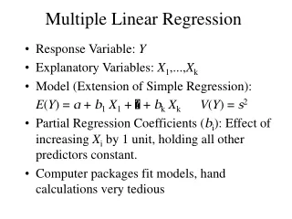
3.3 Hypothesis Testing in Multiple Linear Regression • Questions: • What is the overall adequacy of the model? • Which specific regressors seem important? • Assume the errors are independent and follow a normal distribution with mean 0 and variance 2
3.3.1 Test for Significance of Regression • Determine if there is a linear relationship between y and xj, j = 1,2,…,k. • The hypotheses are H0: β1 = β2 =…= βk = 0 H1: βj 0 for at least one j • ANOVA • SST = SSR + SSRes • SSR/2 ~ 2k, SSRes/2 ~ 2n-k-1, and SSR and SSRes are independent
Under H1, F0 follows F distribution with k and n-k-1 and a noncentrality parameter of
R2 and Adjusted R2 • R2 always increase when a regressor is added to the model, regardless of the value of the contribution of that variable. • An adjusted R2: • The adjusted R2 will only increase on adding a variable to the model if the addition of the variable reduces the residual mean squares.
3.3.2 Tests on Individual Regression Coefficients • For the individual regression coefficient: • H0: βj = 0 v.s. H1: βj 0 • Let Cjj be the j-th diagonal element of (X’X)-1. The test statistic: • This is a partial or marginal test because any estimate of the regression coefficient depends on all of the other regression variables. • This test is a test of contribution of xj given the other regressors in the model
For the full model, the regression sum of square • Under the null hypothesis, the regression sum of squares for the reduce model • The degree of freedom is p-r for the reduce model. • The regression sum of square due to β2 given β1 • This is called the extra sum of squares due to β2 and the degree of freedom is p - (p - r) = r • The test statistic
If β2 0, F0 follows a noncentral F distribution with • Multicollinearity: this test actually has no power! • This test has maximal power when X1 and X2 are orthogonal to one another! • Partial F test: Given the regressors in X1, measure the contribution of the regressors in X2.
Consider y = β0 + β1 x1 + β2 x2 + β3 x3 + SSR(β1| β0 , β2, β3), SSR(β2| β0 , β1, β3) and SSR(β3| β0 , β2, β1) are signal-degree-of –freedom sums of squares. • SSR(βj| β0 ,…, βj-1, βj, … βk) : the contribution of xj as if it were the last variable added to the model. • This F test is equivalent to the t test. • SST = SSR(β1 ,β2, β3|β0) + SSRes • SSR(β1 ,β2 , β3|β0) = SSR(β1|β0) + SSR(β2|β1, β0) + SSR(β3 |β1, β2, β0)
3.3.3 Special Case of Orthogonal Columns in X • Model: y = Xβ + = X1β1+ X2β2 + • Orthogonal: X1’X2 = 0 • Since the normal equation (X’X)β= X’y,
3.3.4 Testing the General Linear Hypothesis • Let T be an m p matrix, and rank(T) = r • Full model: y = Xβ + • Reduced model: y = Z + , Z is an n (p-r) matrix and is a (p-r) 1 vector. Then • The difference: SSH = SSRes(RM) – SSRes(FM)with r degree of freedom. SSH is called the sum of squares due to the hypothesis H0: Tβ = 0
Another form: • H0: Tβ = c v.s. H1: Tβ c Then
3.4 Confidence Intervals in Multiple Regression 3.4.1 Confidence Intervals on the Regression Coefficients • Under the normality assumption,
3.4.2 Confidence Interval Estimation of the Mean Response • A confidence interval on the mean response at a particular point. • x0 = (1,x01,…,x0k)’ • The unbiased estimator of E(y|x0) :
3.4.3 Simultaneous Confidence Intervals on Regression Coefficients • An elliptically shaped region
Another approach: • is chosen so that a specified probability that all intervals are correct is obtained. • Bonferroni method: Δ= tα/2p, n-p • Scheffe S-method: Δ=(2Fα,p, n-p )1/2 • Maximum modulus t procedure: Δ= uα,p, n-2 is the upper tail point of the distribution of the maximum absolute value of two independent student t r.v.’s each based on n-2 degree of freedom
Example 3.11 The Rocket Propellant Data • Find 90% joint C.I. for β0 and β1 by constructing a 95% C.I. for each parameter.
The confidence ellipse is always a more efficient procedure than the Bonferroni method because the volume of the ellipse is always less than the volume of the space covere3d by the Bonferroni intervals. • Bonferroni intervals are easier to construct. • The length of C.I.: Maximum modulus t < Bonferroni method < Scheffe S-method
3.6 Hidden Extrapolation in Multiple Regression • Be careful about extrapolating beyond the region containing the original observations! • Rectangle formed by ranges of regressors NOT data region. • Regressor variable hull (RVH): the convex hull of the original n data points. • Interpolation: x0 RVH • Extrapolation: x0 RVH
hii of the hat matrix H = X(XX)-1X’are useful in detecting hidden extrapolation. • hmax: the maximum of hii . The point xi that has the largest value of hii will lie on the boundary of RVH • {x | x(XX)-1x ≦ hmax } is an ellipsoid enclosing all points inside the RVH. • Let h00 = x0′(X′X)-1x0 • h00 hmax : inside the RVH and the boundary of RVH • h00 > hmax : outside the RVH
3.7 Standardized Regression Coefficients • Difficult to compare regression coefficients directly. • Unit Normal Scaling: Standardize a Normal r.v.
New model: • There is no intercept. • The least-square estimator of b is
New Model: • The least-square estimator:
It does not matter which scaling we use! They both produce the same set of dimensionless regression coefficient.
3.8 Multicollinearity • A serious problem: Multicollinearity or near-linear dependence among the regression variables. • The regressors are the columns of X. So an exact linear dependence would result a singular X’X
Soft drink data: • Off-diagonal elements are of W’W usually called the simple correlations between regressors.
Variance inflation factors (VIFs): • The main diagonal elements of the inverse of X’X ((W’W)-1 above) • From above two cases:Soft drink: VIF1 = VIF2 = 3.12 and Figure 3.12: VIF1 = VIF2 = 1 • VIFj = 1/(1-Rj) • Rj is the coefficient of multiple determination obtained from regressing xj on the other regressor variables. • If xj is nearly linearly dependent on some of the other regressors, then Rj 1 and VIFj will be large. • Serious problems: VIFs > 10
Figure 3.13 (a): The plan is unstable and very sensitive to relatively small changes in the data points. • Figure 3.13 (b): Orthogonal regressors.
3.9 Why Do Regression Coefficients Have the Wrong Sign? • The reasons of the wrong sign: • The range of some of the regressors is too small. • Important regressors have not been included in the model. • Multicollinearity is present. • Computational errors have been made.