Download
1 / 38
380 likes | 604 Vues
Spatial Analysis cont. Density Estimation, Summary Spatial Statistics, Routing . Density Estimation. Spatial interpolation is used to fill the gaps in a field Density estimation creates a field from discrete objects

E N D
Spatial Analysis cont.Density Estimation, Summary Spatial Statistics, Routing
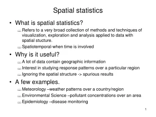
Density Estimation • Spatial interpolation is used to fill the gaps in a field • Density estimation creates a field from discrete objects • the field’s value at any point is an estimate of the density of discrete objects at that point • e.g., estimating a map of population density (a field) from a map of individual people (discrete objects)
Objects to Fields • map of discrete objects and want to calculate their density • density of population • density of cases of a disease • density of roads in an area • density would form a field • one way of creating a field from a set of discrete objects
Density Estimation Using Kernels • Mathematical function • each point replaced by a “pile of sand” of constant shape • add the piles to create a surface
A B (A) A collection of point objects (B) A kernel function for one of the points The kernel’s shape depends on a distance parameter—increasing the value of the parameter results in a broader and lower kernel, and reducing it results in a narrower and sharper kernel. When each point is replaced by a kernel and the kernels are added, the result is a density surface whose smoothness depends on the value of the distance parameter.
Width of Kernel • Determines smoothness of surface • narrow kernels produce bumpy surfaces • wide kernels produce smooth surfaces
Example • Density estimation and spatial interpolation applied to the same data • density of ozone measuring stations vs. • Interpolating surface based on measured levelof ozone at measuring stations
Kernal too small?(radius of 16 km)each kernal isolated from neighbors
A dataset with two possible interpretations: First, a continuous field of atmospheric temperature measured at eight irregularly spaced sample points, and second, eight discrete objects representing cities, with associated populations in thousands. Spatial interpolation makes sense only for the former, and density estimation only for the latter
GEO 565: Best locations for a new Beanerymore factors: proximity to a highway, zoning concerns, income levels, population density, age, etc.
From Transformations to Descriptive Summaries:Summary Spatial Statistics
Descriptive Summaries • Ways of capturing the properties of data sets in simple summaries • mean of attributes • mean for spatial coordinates, e.g., centroid
Spatial Autocorrelation Tobler’s 1st Law of Geography:everything is related to everything else, but near things are more related than distant things S. autocorrelation: formal property that measures the degree to which near and distant things are related. Close in space Dissimilar in attributes Attributes independent of location Close in space Similar in attributes Arrangements of dark and light colored cells exhibiting negative, zero, and positive spatial autocorrelation.
Why Spatial Dependence? • evaluate the amount of clustering or randomness in a pattern • e.g., of disease rates, accident rates, wealth, ethnicity • random: causative factors operate at scales finer than “reporting zones” • clustered: causative factors operate at scales coarser than “reporting zones”
Moran’s Index • positive when attributes of nearby objects are more similar than expected • 0 when arrangements are random • negative when attributes of nearby objects are less similar than expected I = nS S wijcij / SS wijS(zi - zavg)2 n = number of objects in sample i,j - any 2 of the objects Z = value of attribute for I cij = similarity of i and j attributes wij= similarity of i and j locations
Moran’s Indexsimilarity of attributes, similarity of location Dispersed, - SA Extreme negative SA Independent, 0 SA Spatial Clustering, + SA Extreme positive SA
Crime Mapping • Clustering - neighborhood scale
Moran’s Indexsimilarity of attributes, similarity of location Maps from Luc Anselin, University of Illinois U-C, Spatial Analysis Lab
The Local Moran statistic, applied using the GeoDa software (available via geodacenter.asu.edu) to describe local aspects of the pattern of housing value among U.S. states (darker = more expensive) Below avg surrounded by above-avg Oregon, Arizona, Pennsylvania Moran’s I = 0.4011, clustering
Hotspot Analysis, Getis-OrdVideo in 3 Parts • http://bit.ly/cGzF7G • http://bit.ly/a5342O • http://bit.ly/9BFnHa
Fragmentation Statistics • how fragmented is the pattern of areas and attributes? • are areas small or large? • how contorted are their boundaries? • what impact does this have on habitat, species, conservation in general?
1975 1986 1992 Note the increasing fragmentation of the natural habitat as a result of settlement. Such fragmentation can adversely affect the success of wildlife populations.
Fragstats pattern analysis for landscape ecology See GEO 580 site for direct links
FRAGSTATS Overview • derives a comprehensive set of useful landscape metrics • Public domain code developed by Kevin McGarigal and Barbara Marks under U.S.F.S. funding • Exists as two separate programs • AML version for ARC/INFO vector data • C version for raster data
FRAGSTATS Fundamentals • PATCH… individual parcel (Polygon) A single homogeneous landscape unit with consistent vegetation characteristics, e.g. dominant species, avg. tree height, horizontal density ,etc. A single Mixed Wood polygon (stand) CLASS… sets of similar parcels LANDSCAPE… all parcels within an area
FRAGSTATS Fundamentals PATCH… individual parcel (Polygon) • CLASS… setsof similar parcels All Mixed Wood polygons (stands) LANDSCAPE… all parcels within an area
FRAGSTATS Fundamentals PATCH… individual parcel (Polygon) CLASS… sets of similar parcels • LANDSCAPE… all parcels within an area “of interacting ecosystems” e.g., all polygons within a given geographic area (landscape mosaic)
FRAGSTATS Output Metrics • Area Metrics (6), • Patch Density, Size and Variability Metrics (5), • Edge Metrics (8), • Shape Metrics (8), • Core Area Metrics (15), • Nearest Neighbor Metrics (6), • Diversity Metrics (9), • Contagion and Interspersion Metrics (2) • …59 individual indices (US Forest Service 1995 Report PNW-GTR-351)
More Spatial Statistics Resources • GeoDA (geodacenter.asu.edu) • S-Plus • Alaska USGS freeware (www.absc.usgs.gov/glba/gistools/) • Central Server for GIS & Spatial Statistics on the Internet • www.ai-geostats.org • GEO 541 – Spatio-Temporal Variation in Ecology & Earth Science