Download
1 / 31
310 likes | 453 Vues
Lecture 10 1: Project “ Starter ” activity, continued 2: Detectors and the Signal to Noise Ratio. Claire Max Astro 289, UC Santa Cruz February 7, 2013. Part 2: Detectors and signal to noise ratio. Detector technology Basic detector concepts Modern detectors: CCDs and IR arrays

E N D
Lecture 101: Project “Starter” activity, continued2: Detectors and the Signal to Noise Ratio Claire Max Astro 289, UC Santa Cruz February 7, 2013
Part 2: Detectors and signal to noise ratio • Detector technology • Basic detector concepts • Modern detectors: CCDs and IR arrays • Signal-to-Noise Ratio (SNR) • Introduction to noise sources • Expressions for signal-to-noise • Terminology is not standardized • Two Keys: 1) Write out what you’re measuring. 2) Be careful about units! • Work directly in photo-electrons where possible
References for detectors and signal to noise ratio • Excerpt from “Electronic imaging in astronomy”, Ian. S. McLean (1997 Wiley/Praxis) • Excerpt from “Astronomy Methods”, Hale Bradt (Cambridge University Press) • Both are on eCommons
Early detectors: Eyes, photographic plates, and photomultipliers • Eyes • Photographic plates • very low QE (1-4%) • non-linear response • very large areas, very small “pixels” (grains of silver compounds) • hard to digitize • Photomultiplier tubes • low QE (10%) • no noise: each photon produces cascade • linear at low signal rates • easily coupled to digital outputs Credit: Ian McLean
Modern detectors are based on semiconductors • In semiconductors and insulators, electrons are confined to a number of specific bands of energy • “Band gap" = energy difference between top of valence band and bottom of the conduction band • For an electron to jump from a valence band to a conduction band, need a minimum amount of energy • This energy can be provided by a photon, or by thermal energy, or by a cosmic ray • Vacancies or holes left in valence band allow it to contribute to electrical conductivity as well • Once in conduction band, electron can move freely
Bandgap energies for commonly used detectors • If the forbidden energy gap is EG there is a cut-off wavelength beyond which the photon energy (hc/λ) is too small to cause an electron to jump from the valence band to the conduction band Credit: Ian McLean
CCD transfers charge from one pixel to the next in order to make a 2D image rain conveyor belts bucket • By applying “clock voltage” to pixels in sequence, can move charge to an amplifier and then off the chip
Schematic of CCD and its read-out electronics • “Read-out noise” injected at the on-chip electron-to-voltage conversion (an on-chip amplifier)
CCD readout process: charge transfer • Adjusting voltages on electrodes connects wells and allow charge to move • Charge shuffles up columns of the CCD and then is read out along the top • Charge on output amplifier (capacitor) produces voltage
Modern detectors: photons electrons voltage digital numbers • With what efficiency do photons produce electrons? • With what efficiency are electrons (voltages) measured? • Digitization: how are electrons (analog) converted into digital numbers? • Overall: What is the conversion between photons hitting the detector and digital numbers read into your computer?
Quantum Efficiency QE: Probability of detecting a single photon incident on the detector Spectral range (QE as a function of wavelength) “Dark Current”: Detector signal in the absence of light “Read noise”: Random variations in output signal when you read out a detector Gain g : Conversion factor between internal voltages and computer “Data Numbers” DNs or “Analog-to-Digital Units” ADUs Primary properties of detectors
Secondary detector characteristics • Pixel size (e.g. in microns) • Total detector size (e.g. 1024 x 1024 pixels) • Readout rate (in either frames per sec or pixels per sec) • Well depth (the maximum number of photons or photoelectrons that a pixel can record without “saturating” or going nonlinear) • Cosmetic quality: Uniformity of response across pixels, dead pixels • Stability: does the pixel response vary with time?
CCD phase space • CCDs dominate inside and outside astronomy • Even used for x-rays • Large formats available (4096x4096) or mosaics of smaller devices. Gigapixel focal planes are possible. • High quantum efficiency 80%+ • Dark current from thermal processes • Long-exposure astronomy CCDs are cooled to reduce dark current • Readout noise can be several electrons per pixel each time a CCD is read out • Trade high readout speed vs added noise
CCDs are the most common detector for wavefront sensors • Can be read out fast (e.g., every few milliseconds so as to keep up with atmospheric turbulence) • Relatively low read-noise (a few to 10 electrons) • Only need modest size (e.g., largest today is only 256x256 pixels)
What do CCDs look like? Carnegie 4096x4096 CCD Subaru SuprimeCam Mosaic Slow readout (science) Slow readout (science) E2V 80 x 80 fast readout for wavefront sensing
Infrared detectors • Read out pixels individually, by bonding a multiplexed readout array to the back of the photo-sensitive material • Photosensitive material must have lower band-gap than silicon, in order to respond to lower-energy IR photons • Materials: InSb, HgCdTe, ...
Types of noise in instruments • Every instrument has its own characteristic background noise • Example: cosmic ray particles passing thru a CCD knock electrons into the conduction band • Some residual instrument noise is statistical in nature; can be measured very well given enough integration time • Some residual instrument noise is systematic in nature: cannot easily be eliminated by better measurement • Example: difference in optical path to wavefront sensor and to science camera • Typically has to be removed via calibration
Statistical fluctuations = “noise” • Definition of variance: where m is the mean, n is the number of independent measurements of x, and the xi are the individual measured values • If x and y are two independent variables, the variance of the sum (or difference) is the sum of the variances:
Main sources of detector noise for wavefront sensors in common use • Poisson noise or photon statistics • Noise due to statistics of the detected photons themselves • Read-noise • Electronic noise (from amplifiers) each time CCD is read out • Other noise sources (less important for wavefront sensors, but important for other imaging applications) • Sky background • Dark current
Photon statistics: Poisson distribution • CCDs are sensitive enough that they care about individual photons • Light is quantum in nature. There is a natural variability in how many photons will arrive in a specific time interval T , even when the average flux F (photons/sec) is fixed. • We can’t assume that in a given pixel, for two consecutive observations of length Tint, the same number of photons will be counted. • The probability distribution for N photons to be counted in an observation time T is
Properties of Poisson distribution • Average value = FTint • Standard deviation = (FTint)1/2 • Approaches a Gaussian distribution as N becomes large Horizontal axis: FTint Credit: Bruce Macintosh
Properties of Poisson distribution Horizontal axis: FTint Credit: Bruce Macintosh
Properties of Poisson distribution • When < FTint> is large, Poisson distribution approaches Gaussian • Standard deviations of independent Poisson and Gaussian processes can be added in quadrature Horizontal axis: FTint Credit: Bruce Macintosh
How to convert between incident photons and recorded digital numbers ? • Digital numbers outputted from a CCD are called Data Numbers (DN) or Analog-Digital Units (ADUs) • Have to turn DN or ADUs back into microvolts electrons photons to have a calibrated system where QE is the quantum efficiency (what fraction of incident photons get made into electrons), g is the photon transfer gain factor (electrons/DN) and b is an electrical offset signal or bias
Look at all the various noise sources • Wisest to calculate SNR in electrons rather than ADU or magnitudes • Noise comes from Poisson noise in the object, Gaussian-like readout noise RN per pixel, Poisson noise in the sky background, and dark current noise D • Readout noise: where npix is the number of pixels and R is the readout noise • Photon noise: • Sky background: for BSky e-/pix/sec from the sky, • Dark current noise: for dark current D (e-/pix/sec)
Dark Current or Thermal Noise: Electrons reach conduction bands due to thermal excitation Science CCDs are always cooled (liquid nitrogen, dewar, etc.) Credit: Jeff Thrush
Total signal to noise ratio where F is the average photo-electron flux, T is the time interval of the measurement, BSky is the electrons per pixel per sec from the sky background, D is the electrons per pixel per sec due to dark current, and RN is the readout noise per pixel.
Some special cases • Poisson statistics: If detector has very low read noise, sky background is low, dark current is low, SNR is • Read-noise dominated: If there are lots of photons but read noise is high, SNR is If you add multiple images, SNR ~ ( Nimages )1/2
Typical noise cases for astronomical AO • Wavefront sensors • Read-noise dominated: • Imagers (cameras) • Sky background limited: • Spectrographs: Low spectral resolution – background limited; high spectral resolution – dark current limited
Typical noise cases for astronomical AO • Wavefront sensors • CCDs: read-noise dominated: • Seth’s detector wins if or BUT: With Seth’s new detector, there is no read-noise. So wavefront sensor would see only Poisson statistics:
Next time • Laser guide stars (two lectures) • Why are laser guide stars needed? • How do lasers work? • General principles of laser guide star return signal • Two main types of astronomical laser guide stars (Rayleigh and sodium) • Wavefront errors due to laser guide stars