Download
1 / 43
430 likes | 543 Vues
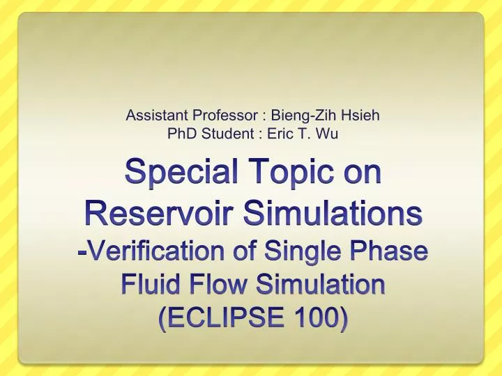
Assistant Professor : Bieng-Zih Hsieh PhD Student : Eric T. Wu. Special Topic on Reservoir Simulations -Verification of Single Phase Fluid Flow Simulation (ECLIPSE 100). Outline. Introduction Purpose Analytical Solution Introduction Introduction of ECLIPSE How to Run a data file

E N D
Assistant Professor : Bieng-Zih Hsieh PhD Student : Eric T. Wu Special Topic on Reservoir Simulations-Verification of Single Phase Fluid Flow Simulation (ECLIPSE 100)
Outline • Introduction • Purpose • Analytical Solution Introduction • Introduction of ECLIPSE • How to Run a data file • How to Find results in 2D • How to Find results in 3D • Results • Homework
Introduction • In the past, our lab had constructed several techniques on reservoir simulations. However, these skills are base on simulators of Computer Modelling Group Ltd (CMGL). • Nowadays, we obtain a new set of much more powerful simulation tools which produced by Schlumberger SIS (ECLIPSE).
Purpose • The purpose of this study is to use ECLIPSE 100 to finish verification of single phase fluid flow simulation.
Analytical Solution Introduction • Assumptions • Slightly compressible liquid, ignorable pressure gradient • Homogeneous, isotropic and isothermal reservoir with uniform thickness • Combine Material Balance and Darcy’s Law • Reservoir at uniform pressure before production • The outer boundary is infinite • Production at constant rate
Analytical Solution Introduction • The solution of diffusion equation is(van Everdingen and Hurst,1949):
GRID Section—Basic Def. Whole Definition • Targets • Grid design(wide, length, thickness, top) • Refine Grid design • Grid property (permeability, porosity) DX 121*10/ DYV 11*10/ DZ 121*10/ EQUALS ‘TOPS’ 3000/ ‘PORO’ 0.17/ ‘PERMX’ 0.01/ / COPY ‘PERMX’ ‘PERMY’ ‘PERMX’ ‘PERMZ’ Define X Direction In here means constant 11 grids 11 grids Setting A=B 1 grid Note: There is no ‘DZV’ keyword in E100 but E300 is.
GRID Section-”EQUALS” EQUALS -- Parameter value ------Box------ -- ‘NAME’ No. I1 I2 J1 J2 K1 K2 ‘TOPS’ 3000 1 11 1 11 1 1/ ‘PORO’ 0.17/--This means all ‘PERMX’ 0.01/ /
GRID Section-”Refine” • Targets: • Refine • Refine Hybrid CARFIN -- Name I1 I2 J1 J2 K1 K2 NX NY NZ ‘REF1’ 5 7 5 7 1 1 9 9 1 / RADFIN -- NAME I J K1 K2 NR NTHETA NZ NWMAX 'Well' 6 6 1 1 10 1 1 1 / RADFIN4 -- NAME I1 I2 J1 J2 K1 K2 NR NTHETA NZ NWMAX ‘Well’ 7 8 7 8 1 1 10 4 1 1 / ENDFIN
PROPS Section • Targets • Relative Permeability • PVT table • Rock properties • Fluid properties • Different phase combinations in the model should obtain different keywords in data file in PROPS section.
PROPS Section-Overview SWOF -- SwKrwKrowPcow / PVTW -- REF.P. FVFW CwREF.VisWViscosibility / ROCK -- REF.P. Cr / DENSITY -- Oil Water Gas / RSCONST -- RS PB / PVCDO -- REF.P FVFO Co VisO /
PROPS Section-RP • Targets • Relative Permeability(SWOF)
PROPS Section-PVT • Targets • PVT table PVTW---Water PVT -- REF.P. REF.FVF CW REF.VISC VISCOSIBILITY 4000 1.029 3.13e-6 0.31 0/ PVCDO---Oil PVT -- REF.P. REF.FVF CW REF.VISC VISCOSIBILITY 4000 1.06 1e-6 13.2 0.0/ RSCONT ---RS=CONST -- RS PB 0.001 1200/
SOLUTION Section-Basic Def. • Target • Reservoir initial conditions EQUIL -- DATUM DATUM OWC OWC GOC GOCRSVD RVVD SOLN -- DEPTH PRESS DEPTH PCOW DEPTH PCOG TABLE TABLEMETH 3050 3600 3300 0 3300 0 1 0 0 /
SUMMARY Section • Targets • Specifies data to be written to the summary file. • Graphics data. • Check keywords in manual to obtain results you want, and write it in your data file. RUNSUM FOPR WGOR ‘PRODUCER’ / WBHP ‘PRODUCER’ /
SCHEDULE Section • Targets • Convergence Condition • Time step (initial, minimum, maximum) • Well specification data • Completion data • Production well control • Time
SCHEDULE Section-Basic Def. IMPES -- == DIMPES by try and error 1.0 1.0 10000.0 / DRSDT – Maximum rate of increase of solution GOR 0 / TUNING 1 1 0.0000001 0.00000001 / 1.0 0.5 1.0E-6 / / WELSPECS -- WELL GROUP LOCATION BHP PI -- NAME NAME I J DEPTH DEFN 'PRODUCER' 'G' 1 1 3050 'OIL' / / COMPDAT -- WELL -LOCATION- OPEN SAT CONN WELL -- NAME I J K1 K2 SHUT TAB FACT DIAM 'PRODUCER' 1 1 1 1 'OPEN' 0 -1 0.5 / / WCONPROD -- WELL OPEN CNTL OIL WATER GAS LIQU RES BHP -- NAME SHUT MODE RATE RATERATERATERATE 'PRODUCER' 'OPEN' 'ORAT‘ 0.1 4* 1000 / / TIME Convergence Condition Well completion data and operation condition Run time
SCHEDULE Section-TIME RPTSCHED 'PRES' 'SOIL' 'SWAT' 'SGAS' 'RS' 'RESTART=2' 'WELLS=2' 'SUMMARY=2' 'CPU=2' 'NEWTON=2' / for 3D view TIME 0.0001
RUNSPEC Section • Targets • Title • Dimension • Grid shape • Phase • Unit • Tables(equilibrium, PVT, well) • Start time • Format
RUNSPEC Section TITLE ODEH PROBLEM - IMPES OPTION - 1200 DAYS DIMENS nr n theta nz-- 10000 1 1 / RADIAL NONNC OIL WATER --Units-- FIELD EQLDIMS 1 100 10 1 1 / TABDIMS 1 1 16 12 / WELLDIMS 1 1 1 1 / NUPCOL 4 / START 19 'OCT' 1982 / NSTACK 24 / FMTOUT FMTIN UNIFOUT UNIFIN
You will see the data is showing in the window then “Run” Note: If it was a wrong choice click the wrong data in the window and click Remove Dataset to remove.
Homework • Simulate a vertical well with different skin factors in an infinite reservoir. • Change your data file from Cartto Radial. • Change your data file from Cart to Cart with LGR. • Change the data file from Oil-water model to Gas-water model. • Verify the results with analytical solutions (only V & H).
GRID Section-”Cart to Radial” • Target: From Cartesian to Radial • RUNSPEC • RADIAL • GRID • DXDN • DYDTHETA • DZDZ • PERMXPERMN • PERMYPERMTHT • PERMZPERMZ • Additional COORDSYS COORDSYS -- K1 K2 Completed 1 1 COMP/ --COMP Means circle complete by definition(total should be 360) above, if it is not a complete circle, use INCOMP instead. --There is other way to define radial model, using keywords “INRAD” and “OUTRAD.”