Download

1 / 27
270 likes | 547 Vues
INDE 2333 ENGINEERING STATISTICS I GOODNESS OF FIT. University of Houston Dept. of Industrial Engineering Houston, TX 77204-4812 (713) 743-4195. AGENDA. Chi-square goodness of fit test. GOODNESS OF FIT TESTS.

E N D
INDE 2333 ENGINEERING STATISTICS I GOODNESS OF FIT University of Houston Dept. of Industrial Engineering Houston, TX 77204-4812 (713) 743-4195
AGENDA • Chi-square goodness of fit test
GOODNESS OF FIT TESTS • Used to determine if a sample could have come from a distribution with the specified parameters • Commonly used to determine if data is normally distributed • Many tests such as the ones that we have been using require normally distributed data. • If data is not normally distributed, non-parametric tests must be used (next subject in the course) • Also used for input distributions in system modeling • Customers or jobs arrive exponentially distributed? • Service times follow what distribution? • Failures occur according to what distribution?
GOODNESS OF FIT TESTS • Based on a comparison of observations between • Observed data • Theoretical data • The comparison utilizes a set of intervals or cells • Each cell has a lower and upper boundary values • The determination of the boundaries are a function of • Theoretical distribution • Number of observations in the sample • 2 different approaches…
TWO DIFFERENT APPROACHES • Approach 1 • Used in the book • Equal interval approach • No cell grouping can have less than 5 expected observations • Approach 2 • Used in other books • Equiprobable approach • Maximum number of cells not to exceed 100 such that the expected number of observations is at least 5 = Int ( obs/5 ) • Expected number of obs in each cell = obs / cells • More statistically robust
HYPOTHESES TEST PROCEDURE • Identify Ho and Ha • Determine level of significance (generally 0.05 or 0.01) • Determine “critical value” criterion from level of significance • Calculate “test statistic” • Make decision • Fail to reject Ho • Reject Ho
HYPOTHESES • Ho • The sample could have come from a distribution with the specified parameters • Ha • The sample could not have come from a distribution with the specified parameters
CRITICAL VALUE • Chi-square distribution chart • One sided test • Alpha typically 0.05 • Degrees of freedom • # of cells - # of parameters used from sample -1 • The -1 is always used due to the known sample size n • Note, if the parameters are specified not sampled then they do not reduce the number of degrees of freedom in the above equation
CHI-SQUAREfor a particular number of degrees of freedom f(X^2) Right tail probability, alpha, typically 0.05 0 X^2 X^2 Critical value
DECISION • Cannot reject • Test statistic is less than the critical value • Sample could have come from a distribution with the specified parameters • Reject • Test statistic is greater than the critical value • Sample could not have come from a distribution with the specified parameters
EXAMPLE 1EQUAL INTERVAL APPROACH • 400 5 minute intervals were observed for air traffic control messages • At alpha=0.01, is the distribution of the number of messages able to be considered as having a poisson distribution with a mean of 4.6? • Approach • Lamba parameter of 4.6 is given • Use the poisson table probability table for 4.6 • Multiply the probability by 400 to obtain the expected observations • Compare the actual observations to the expected observations
HYPOTHESES • Ho: • Poisson distribution with mean of 4.6 • Ha: • Not poisson distribution with a mean of 4.6
CHI-SQUAREfor 10-1 degrees of freedom f(X^2) Right tail probability, alpha = 0.01 0 X^2 16.919 Critical value
DECISION • Test statistic of 6.749 is less than the critical value of 16.919 • Cannot reject Ho of distribution being poisson with a mean of 4.6 • There is evidence to support the claim that the data came from a poisson distribution with a mean of 4.6 at an alpha level of 0.01
EXAMPLE 2EQUIPROBABLE APPROACH • Were the scores from an INDE 2333 exam normally distributed? • Sample statistics • Mean=71.95 • Std=11.93 • N=43
HYPOTHESES • Ho • The sample could have come from a normally distributed population with a mean of 71.95 and a std of 11.93 • Ha • The sample could not have come from a normally distributed population with a mean of 71.95 and a std of 11.93
CRITICAL VALUE • Chi-square distribution chart • One sided test • 0.05 • Degrees of freedom • The sample size is 43 • Want the maximum number of cells not to exceed 100 with a minimum expected number of observation of 5 • 43/5=8.6 cells • With 8 cells, the expected number of observations is 5.375 • Degrees of freedom is number of cells – number of parameters used from sample-1 • Degrees of freedom=8-2-1=5
CHI-SQUAREfor 5 of degrees of freedom f(X^2) 0.05 0 X^2 11.070
CELL BOUNDARIES • To calculate observed values in each cell, we must determine the actual x cell boundaries from the 8 equiprobable cells • For normal distributions • Look up z value corresponding to probability • Boundaries =mean+std * Z
DECISION • 2.581 < 11.070 • Cannot reject the Ho • Evidence to support the claim that the test scores are normally distributed with a mean of 71.95 and std of 11.93
IN EXCEL • Frequency • Data_array, bins_array • Range operation • CTRL-SHIFT-ENTER • Norminv function • Probability, mean, std • Chiinv function • Probability, df