Download
1 / 25
260 likes | 453 Vues
Chapter 13. Black / Scholes Model. I. Limiting Case of N-Period Binomial Model. A. If we let N , split the time until exp . ( e.g. 1 year ) into shorter intervals , until S moves continuously . Then Binomial Model reduces to Black / Scholes Model.

E N D
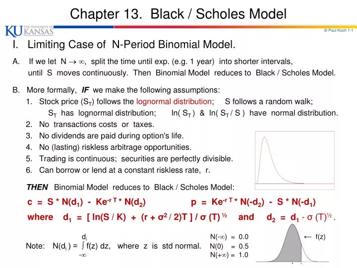
Chapter 13. Black / Scholes Model I. Limiting Case of N-Period Binomial Model. A. If we let N , split the time until exp. (e.g. 1 year) into shorter intervals, until S moves continuously. Then Binomial Model reduces to Black / Scholes Model. B. More formally, IF we make the following assumptions: 1. Stock price (ST) follows the lognormal distribution; S follows a random walk; ST has lognormal distribution; ln( ST ) & ln( ST / S ) have normal distribution. 2. No transactions costs or taxes. 3. No dividends are paid during option's life. 4. No (lasting) riskless arbitrage opportunities. 5. Trading is continuous; securities are perfectly divisible. 6. Can borrow or lend at a constant riskless rate, r. THEN Binomial Model reduces to Black / Scholes Model: c = S * N(d1) - Ke-r T * N(d2) p = Ke-r T * N(-d2) - S * N(-d1) where d1= [ ln(S / K) + (r + σ2 / 2)T ] / σ (T) ½ and d2= d1- σ (T)½ . diN(-) = 0.0 ← f(z) Note: N(di ) = ∫ f(z) dz, where z is stdnormal. N(0) = 0.5 - N(+) = 1.0
II. Comparing Black / Scholes with N-Pd Binomial Model N-PdBinomial Model: c = S * B[a,n,p'] - Ke-rT* B[a,n,p] ↓↓ Black/Scholes Model: c = S * N(d1) - Ke-rT* N(d2) A. Cox, Ross, and Rubinstein (JFE, 1979) show that, as n , B[a,n,p'] N(d1) and B[a,n,p] N(d2), and the two formulas converge. Thus, we can use same intuition as the Binomial Model. Call value is the expected payoff of the option discounted back to the present at the riskless rate.
II. Comparing Black / Scholes with N-Pd Binomial Model Black/Scholes Model: c = S * N(d1) - Ke-r T * N(d2) p = Ke-r T * N(-d2) - S * N(-d1) B. More Intuition: 1. Recall, lower bound for call: c S - Ke-r T 2. Recall, lower bound for put: p Ke-r T - S 3. Observe that Black / Scholes formula for a call weights: S by N(d1) and Ke-r Tby N(d2). 4. S is weighted by N(d1), which is the hedge ratio, Δ. [ Hedge portfolio contains N(d1) shares for each call written.] 5. Ke-r T is weighted by N(d2), which is the probability that call will finish ITM in a risk-neutral world. 6. Thus, the Black/Scholes formula can be interpreted as: [ Stock Price multiplied by hedge ratio (# shares you’ll own) ] minus [ NPV (K) multiplied by probability that you’ll pay K {P(call ITM)} ].
II. Comparing Black / Scholes with N-Pd Binomial Model Black/Scholes Model: c = S0* N(d1) - Ke-rT* N(d2) C. Even More Intuition: 1. N(d1) is hedge ratio (# shares of stock for each call sold in hedge pf). 2. {S0 N(d1)e rT} is expected stock value at time T in a risk-neutral world, when all possible values of S < K are counted as zero (OTM). 3. N(d2) is probability that call will be exercised in a risk-neutral world. 4. The strike price (K) is only paid if call is ITM ( with probability, N(d2) ). 5. Thus, call has the following future expected value in a risk-neutral world: E(c) = {S0 N(d1) erT} - K * N(d2). 6. Discounting this expression to the present, we get: E(c) e-rT = {S0 N(d1)} - Ke -rT * N(d2) . Thus, value of call today is expected future value of call, discounted back.
II. Comparing Black / Scholes with N-Pd Binomial Model Black/Scholes Model: c = S0* N(d1) - Ke-rT* N(d2) D. Even MoreIntuition: 1. The equation above can be multiplied and divided by { e-rT*N(d2) }: c = e-rT* N(d2) [ S0 erT* N(d1) / N(d2) - K ] 2. The terms in this expression have the following interpretation: a. e-rT: Present value NPV factor; b. N(d2) : Probability of exercise (i.e., that S > K); c. e-rT* N(d1) / N(d2) : Expected percentage increase in stock if option is exercised (i.e., if S > K); d. K : Strike price paid if option is exercised (i.e., if S > K). 3. So, call value = NPV of expected value of purchase if option exercised.
III. Properties of Black / Scholes Formulas c = S * N(d1) - Ke-r T * N(d2) p = K e-r T * N(-d2) - S * N(-d1) where d1= [ ln(S/K) + (r + σ2/2)T ] / σ (T)½ and d2 = d1 - σ (T)½ . A. When ST gets large, call will likely be exercised. 1. Then European call is similar to forward contract for F = K. Then right to buy acts like a promise to buy. 2. Then value of call is analogous to value of forward: c = S - Ke-r T is analogous to f = S - Ke-r T. (ST large; d1 large; N(d1) 1.) 3. This is price given by B / S Formula; when S becomes large, d1and d2 become large, so that N(d1) and N(d2) both 1. B. When ST gets large, put will not be exercised. 1. Put value goes toward zero. 2. This is price given by B / S Formula; when S becomes large, d1 and d2 become large, so that N(-d1) and N(-d2) both 0.
III. Properties of Black / Scholes Formulas c = S * N(d1) - Ke-r T * N(d2) p = K e-r T * N(-d2) - S * N(-d1) where d1 = [ ln(S/K) + (r + σ2/2)T ] / σ (T)½ and d2 = d1 - σ (T)½ . C. When volatility (σ) goes to 0, stock is virtually riskless, and E(ST) SerT, so that payoff from call is max { SerT- K, 0 }. 1. Discounting this payoff at r, today's call value is: e -rTmax { SerT- K, 0 } = max { S - Ke -rT, 0 }. 2. To show this is consistent with B / S Formulas, consider two cases: i. S > Ke -rT; then ln(S/ K) + rT > 0; as σ 0, d1 & d2 +, so that N(d1) & N(d2) 1, and c S - Ke-r T ; ii. S < Ke -rT; then ln(S/ K) + rT < 0; as σ 0; d1 & d2 -, so that N(d1) & N(d2) 0, and c 0.
III. Properties of Black / Scholes Formulas D. Recallfrom Chapter 12 - Risk Neutral Valuation 1. Consider the expected return from the stock, when the probability of an up move is assumed to be p. E(ST) = pSu + (1-p)Sd E(ST) = pS(u-d) + Sd[subst. p = (erT- d) / (u-d)] E(ST) = (erT- d) S(u-d) / (u-d) + Sd E(ST) = (erT- d) S + Sd E(ST) = erTS a. On average the stock price grows at the riskfreerate. b. Setting the probability of an up move equal to p is the same as assuming the stock earns the riskfreerate. c. If investors are risk-neutral, they require no compensation for risk, and the expected return on all securities is the riskfree rate.
III. Properties of Black / Scholes Formulas 2. The Risk-Neutral Valuation Principle. a. Any option can be valued on the assumption that the world is risk-neutral. b. To value an option, we can assume: i. expected return on all traded securities is r; ii. the P.V. of expected future cash flows can be valued by discounting at r. c. The prices we get are correct, not just in a risk-neutral world, but in other worlds as well. d. Risk-Neutral Valuation works because you can always get a hedge portfolio using options, so arbitrageurs force the option value to behave this way.
III. Properties of Black / Scholes Formulas E. The Riskfree Rate (r) is important in B / S Model. 1. B / S assumes r is constant. In practice use Treasury rate or LIBOR Zero rate for same maturity as option. 2. B / S does NOT depend on: a. Individual risk preferences (attitudes toward risk); b. Expected Return on underlying stock (e.g., from CAPM). 3. 2.a & b result from following fact: a. Option prices are determined from arbitrage conditions. b. Hedge portfolio provides investment opportunity with no risk. 4. This fact also leads to Risk Neutral Valuation Principle: a. Any security that is dependent on other traded securities can be priced on the assumption that world is risk neutral. b. This does not state that world is risk neutral! c. Only states that options can be valued on this assumption. 5. THUS: Investors’ risk preferences do not affect value of options. Value of options does not depend on stock’s expected return. 6. Powerful result. Expected return on all securities is riskfreerate (r). r is the appropriate discount rate for all future cash flows. Arbitrage arguments & risk neutral valuation give same result.
III. Properties of Black / Scholes Formulas F. What’s behind the B/S Model? 1. B / S analogous to Binomial Model; Can also be derived using risk neutral valuation. a. Assume stock’s expected return () is r. b. Calculate expected payoff from option at maturity (T). c. Discount expected payoff at r. 2. The math is messy (stochastic calculus). We rely on Binomial Model for intuition. 3. A hedge portfolio can always be set up; Combine shares with 1 short call, a. Works because S & c are affected by the same source of uncertainty →S. b. In any short period of time (if r & constant), S & c (and S & p) move proportionately; i.e., (S,c) = 1 and (S,p) = -1. c. Thus, when hedge portfolio is set up, gain / loss on stock is exactly offset by loss / gain on the option; so value of hedge portfolio is known with certainty. 4. Example: Suppose c = (.5)S (c is prop. to S). Then hedge ratio, = .5! Buy =.5 share, sell 1 call. c (or buy 1 share, sell 2 calls). (slope = .5) This pf is riskless pay r! (∆ = dc/dS) Now formula has 1 unknown; Can solve for c = f (S,K,r,T,).______________________S K
III. Properties of Black / Scholes Formulas G. Important difference between Binomial & B / S Models. 1. With Binomial Model, hedge ratio is fixed. For one period model, = (cu – cd) / (Su – Sd). For N – period model, = 1 / B( a,N,p’ ). Given the other parameters, does not change. 2. With B / S Model, hedge portfolio is riskless only briefly. The hedge ratio changes over time. If = .5 today, it may be .4 tomorrow. Then hedge portfolio must be adjusted over time. Dynamic Hedging strategies! (Chapter 17).
IV. The Lognormal Distribution for ST A. Usual assumption: S follows a random walk; 1. St= St-1 + εt; or St- St-1 = εt. (εt is Normally distributed) 2. This implies: a. Returns on S over a short time (Δt) are normally distributed; b. ST = stock price at future time, T, has lognormal distribution. │ │ │ │ │ ln(ST/S) │ ST 0 0 Normal Lognormal Normal ranges between -& + ; Lognormal is > 0.
IV. The Lognormal Distribution for ST B. If ST ~ Lognormal, then ln(ST) ~ Normal. 1. In fact, ln(ST) ~ N { ln S + (μ - σ2 / 2) T, σ(T) ½ }, a. μ = Expected return from stock ( r!); b. σ = Volatility of stock return. i. Measure of uncertainty about Return on S; ii. Defined so that σ(Return on S) in period (Δt) is σΔt . 2. Thus, E [ ln( ST ) ] = ln S + (μ - σ2 / 2) T; Var( ln ST ) = σ2T. 3. Note: ln(ST/S) is continuously compounded return over T; a. ln(ST / S ) ~ N { (μ - σ2 / 2) T, σ(T) ½ }.
IV. The Lognormal Distribution for ST 4. This follows from the distribution of ln(ST ); a. E[ ln(ST ) ] = ln S + (μ - σ2 / 2) T ; So E[ ln(ST / S ) ] = E[ ln(ST ) ] - ln S = (μ - σ2 / 2) T . 5. Interpretation: Letting T = 1 year, The continuously compounded return on S has mean (μ - σ2/2) and standard deviation σ. 6. What about the level of ST? It turns out that: a. E( ST ) = S eμ T & Var( ST ) = S2 e 2μ T (eσ2 T - 1). b. This conforms to our definition that μ = expected return on S.
IV. The Lognormal Distribution for ST C. Consider Expected Return of Lognormal ST. 1. According to CAPM, the expected return on stock, μ, depends on riskfree return and riskiness of stock (β). 2. But we don't have to worry about determinants of μ ; Because of the risk-neutral valuation principle, the value of an option on ST does not depend on μ. 3. E[ ln(ST / S )] = (μ - σ2 / 2) T < μT! [Why not μ?] Annualized expected return continuously compounded over period T is less than μ, which is the annualized expected return in a short time period .
IV. The Lognormal Distribution for ST 4. Example: Consider following sequence of annual returns, { 15%, 20%, 30%, -20%, 25% }, for 5 years. Arithmetic mean = (1/5)Σ ri = 14.0% . Geometric mean = [ Π (1+ri) ]1/5 - 1 = 12.4% . a. If we use annual compounding, earn Geometric mean. b. Fact: Unless annual returns are the same each year, Geometric mean < Arithmetic mean. Thus, the Lognormal distribution has the correct mean. 5. The Point: Annualized expected return compounded over pdT Annualized expected return in short time pd, Δt(μ). a. That is, (μ - σ2 / 2) T < μT or (μ - σ2 / 2) < μ. 6. This shows that the term, “expected return,” is ambiguous: either μ or (μ-σ2 / 2); compounded over T, or instantaneous over Δt.
IV. The Lognormal Distribution for ST D. Consider Annualized Volatilityof Lognormal ST -- σ. 1. A measure of uncertainty about stock returns. a. Std Dev of continuously compounded return on stock over 1 year, b. Often expressed as % per annum. c. “Old economy stocks” σ ranges from .2 to .4 (20% - 40%). d. “New economy stocks” ranges from .4 to .6 (40% - 60%). 2. Rough approximation: σ (T) ½ is the Std Dev of stock return over time T. a. Suppose σ = 30%, and T = .5 (6 months); b. The Std Dev of return in 6 months is σ (T) ½ = 30 (.5) ½ = 21.2%; c. The Std Dev of return in 3 months is σ (T) ½ = 30 (.25) ½ = 15.0%; --- and so on. 3. The “square root effect” is important in assessing risk. a. In general, uncertainty about ST increases as the square root of how far ahead we are looking.
V. Problem: Must Estimate Volatility (σ) A. Use Historical Data on Si(Historical Volatility). 1. Define: n = # of observations on Si , and on xi = ln(Si / Si-1 ) returns; Si = stock price at end of ith interval; τ = length of time interval (e.g., daily, weekly, … ). Let = [1 / (n-1) Σ(xi - x)2] ½ = Std Dev of Return over interval, τ. 2. Let τ = 1 day; then xi = ln(Si / Si-1 ) dailyreturns; for 1 year. a. Then estimates volatility over one day. b. Multiplythis estimate by (252)½ to get annualized volatilityof ST, for input to B / S Model. The stderror of is [ (252) ½ / (2n) ½ ]. d. There are 252 trading days in 1 year. (Ignore non-trading days.) 3. Let τ = 1 week; then xi = ln(Si / Si-1 ) weeklyreturns; for 1 year. a. Then estimates volatility over one week. b. Multiplythis estimate by(52)½ to get annualized volatilityof ST, 4. Problem: σ may not be constant for entire year. a. Common Practice: use daily closing prices from past 90 days.
V. Problem: Must Estimate Volatility (σ) B. Implied Volatility. 1. Black / Scholes formula shows how: c = f ( S, K, T, r, σ, D). 2. At any time, we knowcurrent values of S, K, T, r, & D. Don’t know σ. 3. Since we also know the current value of the option (c), we can plug in the current value of c on the left-hand-side, and the current values of S, K, T, r, & D on the right-hand-side, and solve for the value of σ that gives today’s value, c. 4. This value of σ is the implied volatility of the current option price; the value of σ that would lead to today’s value of the option. 5. Forward - looking measure of σ; What option traders think σ will be over life of option, to get c ! 6. Easy to compute. See my excel program.
V. Problem: Must Estimate Volatility (σ) C. VIX. 1. The CBOE publishes indexes that track implied volatility in markets. 2. Most popular index: the SPX VIX. a. An index of avgimplied volatility of 30-day options on the S&P 500. b. Calculated from a wide range of calls & puts with different K’s & T’s. c. If VIX = 15, means implied volatility of 30-day options on S&P 500 is about 15%, on average. 3. Can trade futures on VIX; different bet than trading options on S&P 500; a. Future value of options on S&P 500 depends onlevel & σof S&P 500. b. Futures on VIXdepends only on σof S&P 500. 4. Indicates what market believes future σ will be (what they pay for options!) Called the “Fear Factor.” See Figure; tracks VIX since 2004.
V. Problem: Must Estimate Volatility (σ) C. VIX. The VIX Index of S&P 500 Implied Volatility; Jan. 2004 - Sept. 2012
VI. Dividends A. If there is no dividendpaid during life of option, then B / S Model works for European or American calls and for European puts. B. What if there is a dividend? 1. Let D = NPV(expected dividends during life of option). 2. When stock goes ex-dividend, S should by roughly D. 3. Assume: Can predict how far S will on ex-date. This is the amount we mean by D. This S should c (or C) and p (or P). C. European options on a dividend-paying stock. 1. Assume S = the sum of two components: Riskless Component = D and Risky Component = remainder of S, (S - D). 2. Procedure: Subtract Riskless Component, & use Risky Component in B / S model: c = (S - D) * N(d1) - K e-r T * N(d2)p = K e-r T * N(-d2) - (S - D) * N(-d1) 3. Intuition: European options can only be exercised at maturity; don’t get div. get (S-D). can subtract D from S and use B / S Model as if stock did not pay dividend.
VI. Dividends D. American Options on a dividend-paying stock. 1. American call may be exercised early if there is a dividend paid during its life. 2. Early exercise of American call is more likelyif: a. D is larger; ← (more to gain) b. (S - K) is larger (more ITM); ← (less extrinsic value to lose) c. Ex-div date closer to expiration. ←(smaller T remaining) 3. Then it may be worth exercising & foregoing remaining extr. value, to avoid the S (loss in intrinsic value) on ex-div. date. 4. Such a call will most likely be exercised just before ex-div. date.
VI. Dividends E. Black's Approximation for pricing American calls. 1. Calculate the price of 2 European calls: a. One matures at T (same time as American call); b. Other matures just before ex-dividend date, at Td < T. (If there is >1 dividend paid, then consider the maturity just before the last ex-div. date.) 2. For 1.a., do dividend adjustment to S, as in VI.C. above. That is, use (S - D) in formula. Euro! You don’t get dividend! 3. Do not make this adjustment for 1.b. You get dividend! Other parameters are same for 1.a & 1.b. 4. Then let the price of American call be the larger of these two European option prices.