Download
1 / 46
460 likes | 606 Vues
2IL50 Data Structures. Spring 2014 Lecture 1: Introduction. Algorithms. Algorithm a well-defined computational procedure that takes some value, or a set of values, as input and produces some value, or a set of values, as output.

E N D
2IL50 Data Structures Spring 2014Lecture 1: Introduction
Algorithms Algorithma well-defined computational procedure that takes some value, or a set of values, as input and produces some value, or a set of values, as output. Algorithmsequence of computational steps that transform the input into the output. Algorithms researchdesign and analysis of algorithms and data structures for computational problems.
Data structures Data Structurea way to store and organize data to facilitate access and modifications. Abstract data typedescribes functionality (which operations are supported). Implementationa way to realize the desired functionality • how is the data stored (array, linked list, …) • which algorithms implement the operations
The course • Design and analysis of efficient algorithms for some basic computational problems. • Basic algorithm design techniques and paradigms • Algorithms analysis: O-notation, recursions, … • Basic data structures • Basic graph algorithms
Some administration first before we really get started …
Organization Lecturer: Prof. Dr. Bettina Speckmann, MF 6.094, b.speckmann@tue.nl I’mhereeverydaybutFriday … Web page: http://www.win.tue.nl/~speckman/2IL50.html Book: T.H. Cormen, C.E. Leiserson, R.L. Rivest and C. Stein.Introduction to Algorithms (3rd edition)mandatory
Prerequisites • Being able to work with basic programming constructs such as linked lists, arrays, loops … • Being able to apply standard proving techniques such as proof by induction, proof by contradiction ... • Being familiar with sums and logarithms such as discussed in Chapter 3 and Appendix A of the textbook. • If you think you might lack any of this knowledge, please come and talk to me immediately so we can get you caught up.
Grading scheme 2IL50 • 6 homework assignments, the best 5 of which each count for 10% of the final grade. • A written exam (closed book) which counts for the remaining 50% of the final grade. • If you reach less than 50% of the possible points on the homework assignments, then you are not allowed to participate in the final exam nor in the second chance exam. You will fail the course and your next chance will be next year. Your grade will be the minimum of 5 and the grade you achieved. If you reach less than 50% of the points on the final exam, then you will fail the course, regardless of the points you collected with the homework assignments. However, you are allowed to participate in the second chance exam. The grade of the second chance exam replaces the grade for the first exam, that is, your homework assignments always count for 50% of your grade. Do the homework assignments!
Homework Assignments • Posted on web-page on Monday before lecture. • Due Sundays at 23:59 as .pdf in the electronic mailbox of your instructor. • Late assignments will not be accepted. Only 5 out of 6 assignments count, hence there are no exceptions. • Must be typeset – use Latex! See example file on web-page. • Name scheme: Ai-LastName.pdf. If your name is Anton van Gelderland and you submit the 1st assignment, then your file must be named A1-vanGelderland.pdf. • Use the tag [2IL50] in the subject line of your email. Any questions: Stop by my office whenever you want (except Fridays!) (send email if you want to make sure that I have time)
Academic Dishonesty Academic DishonestyAll class work has to be done independently. You are of course allowed to discuss the material presented in class, homework assignments, or general solution strategies with me or your classmates, but you have to formulate and write up your solutions by yourself. You must not copy from the internet, your friends, or other textbooks. Problem solving is an important component of this course so it is really in your best interest to try and solve all problems by yourself. If you represent other people's work as your own then that constitutes fraud and will be dealt with accordingly.
Organization Components: • Lectures Monday 5+6 AUD 1 Wednesday 3+4 AUD 1 • LabMonday 7+8 AUD 3You can work on this week's home work assignment. Several of the instructors will be present to answer questions. • Tutorials Wednesday 1+2 see web-page for rooms and instructors!The instructors will explain the solutions to the homework assign-ments of the previous week and answer any questions that arise. • Check web-page for details
Signing up • You should have registered by 12-01-2014. • One more opportunity: register on OASE by Monday, 03-02-2014, 20:00. That’s today! • You can not register for groups yet, that will follow tonight at 21:00!
Sorting let’s get started …
The sorting problem Input: a sequence of n numbers ‹a1, a2, …, an› Output: a permutation of the input such that ‹ai1≤ … ≤ain› • The input is typically stored in arrays • Numbers ≈ Keys • Additional information (satellite data) may be stored with keys • We will study several solutions ≈ algorithms for this problem
Describing algorithms • A complete description of an algorithm consists of three parts: • the algorithm (expressed in whatever way is clearest and most concise, can be English and / or pseudocode) • a proof of the algorithm’s correctness • a derivation of the algorithm’s running time
InsertionSort • Like sorting a hand of playing cards: • start with empty left hand, cards on table • remove cards one by one, insert into correct position • to find position, compare to cards in hand from right to left • cards in hand are always sorted InsertionSort is • a good algorithm to sort a small number of elements • an incremental algorithm Incremental algorithmsprocess the input elements one-by-one and maintain the solution for the elements processed so far.
Incremental algorithms Incremental algorithmsprocess the input elements one-by-one and maintain the solution for the elements processed so far. • In pseudocode: IncAlg(A) // incremental algorithm which computes the solution of a problem with input A = {x1,…,xn} • initialize: compute the solution for {x1} • for j = 2 to n • do compute the solution for {x1,…,xj} using the (already computed) solution for {x1,…,xj-1} Check book for more pseudocode conventions no “begin - end”, just indentation
InsertionSort InsertionSort(A) // incremental algorithm that sorts array A[1..n] in non-decreasing order • initialize: sort A[1] • for j = 2 to A.length • do sort A[1..j] using the fact that A[1.. j-1] is already sorted
1 j n 1 3 14 17 28 6 … InsertionSort InsertionSort(A) // incremental algorithm that sorts array A[1..n] in non-decreasing order • initialize: sort A[1] • for j = 2 to A.length • do key = A[j] • i = j -1 • whilei > 0 and A[i] > key • do A[i+1] = A[i] • i ← i -1 • A[i +1] = key InsertionSort is an in place algorithm: the numbers are rearranged within the array with only constant extra space.
Correctness proof • Use a loop invariant to understand why an algorithm gives the correct answer. Loop invariant (for InsertionSort)At the start of each iteration of the “outer” for loop (indexed by j) the subarray A[1..j-1] consists of the elements originally in A[1..j-1] but in sorted order.
Correctness proof • To proof correctness with a loop invariant we need to show three things: InitializationInvariant is true prior to the first iteration of the loop. MaintenanceIf the invariant is true before an iteration of the loop, it remains true before the next iteration. TerminationWhen the loop terminates, the invariant (usually along with the reason that the loop terminated) gives us a useful property that helps show that the algorithm is correct.
Correctness proof InsertionSort(A) • initialize: sort A[1] • for j = 2 to A.length • do key = A[j] • i = j -1 • while i > 0 and A[i] > key • do A[i+1] = A[i] • i = i -1 • A[i +1] = key InitializationJust before the first iteration, j = 2 ➨ A[1..j-1] = A[1], which is the element originally in A[1], and it is trivially sorted. Loop invariantAt the start of each iteration of the “outer” for loop (indexed by j) the subarray A[1..j-1] consists of the elements originally in A[1..j-1] but in sorted order.
Correctness proof InsertionSort(A) • initialize: sort A[1] • for j = 2 to A.length • do key = A[j] • i = j -1 • while i > 0 and A[i] > key • do A[i+1] = A[i] • i = i -1 • A[i +1] = key MaintenanceStrictly speaking need to prove loop invariant for “inner” while loop. Instead, note that body of while loop moves A[j-1], A[j-2], A[j-3], and so on, by one position to the right until proper position of key is found (which has value of A[j]) ➨ invariant maintained. Loop invariantAt the start of each iteration of the “outer” for loop (indexed by j) the subarray A[1..j-1] consists of the elements originally in A[1..j-1] but in sorted order.
Correctness proof InsertionSort(A) • initialize: sort A[1] • for j = 2 to A.length • do key = A[j] • i = j -1 • while i > 0 and A[i] > key • do A[i+1] = A[i] • i = i -1 • A[i +1] = key TerminationThe outer for loop ends when j > n; this is when j = n+1 ➨ j-1 = n. Plug n for j-1 in the loop invariant ➨ the subarray A[1..n] consists of the elements originally in A[1..n] in sorted order. Loop invariantAt the start of each iteration of the “outer” for loop (indexed by j) the subarray A[1..j-1] consists of the elements originally in A[1..j-1] but in sorted order.
Another sorting algorithm using a different paradigm …
MergeSort • A divide-and-conquer sorting algorithm. Divide-and-conquerbreak the problem into two or more subproblems, solve the subproblems recursively, and then combine these solutions to create a solution to the original problem.
Divide-and-conquer • D&CAlg(A) • // divide-and-conquer algorithm that computes the solution of a problem with input A = {x1,…,xn} • if # elements of A is small enough (for example 1) • then compute Sol (the solution for A) brute-force • else • split A in, for example, 2 non-empty subsets A1 and A2 • Sol1 = D&CAlg(A1) • Sol2= D&CAlg(A2) • compute Sol(the solution for A)from Sol1 and Sol2 • return Sol
MergeSort • MergeSort(A) • // divide-and-conquer algorithm that sorts array A[1..n] • if A.length == 1 • then compute Sol (the solution for A) brute-force • else • split A in 2 non-empty subsets A1 and A2 • Sol1 = MergeSort(A1) • Sol2= MergeSort(A2) • compute Sol(the solution for A)from Sol1 en Sol2
MergeSort • MergeSort(A) • // divide-and-conquer algorithm that sorts array A[1..n] • if length[A] = 1 • thenskip • else • n = A.length ; n1= n/2 ; n2= n/2 ; • copy A[1.. n1] to auxiliary array A1[1.. n1] • copy A[n1+1..n] to auxiliary array A2[1.. n2] • MergeSort(A1) • MergeSort(A2) • Merge(A, A1, A2)
3 14 1 28 17 8 21 7 4 35 1 3 4 7 8 14 17 21 28 35 3 14 1 28 17 8 21 7 4 35 1 3 14 17 28 4 7 8 21 35 3 14 1 28 17 3 14 1 17 28 3 14 MergeSort
1 3 14 17 28 4 7 8 21 35 A1 A2 MergeSort • Merging A 1 3 4 7 8 14 17 21 28 35
MergeSort: correctness proof Induction on n (# of input elements) • proof that the base case (n small) is solved correctly • proof that if all subproblems are solved correctly, then the complete problem is solved correctly
MergeSort: correctness proof • MergeSort(A) • if length[A] = 1 • thenskip • else • n = A.length ; n1= n/2 ; n2= n/2 ; • copy A[1.. n1] to auxiliary array A1[1.. n1] • copy A[n1+1..n] to auxiliary array A2[1.. n2] • MergeSort(A1) • MergeSort(A2) • Merge(A, A1, A2) Proof (by induction on n) Base case: n = 1, trivial ✔ Inductive step: assume n > 1. Note that n1< n and n2< n. Inductive hypothesis ➨arrays A1 and A2 are sorted correctly Remains to show: Merge(A, A1, A2)correctly constructs a sorted array A out of the sorted arrays A1 and A2 … etc. ■ Lemma MergeSortsorts the array A[1..n]correctly.
QuickSort another divide-and-conquer sorting algorithm…
QuickSort • QuickSort(A) • // divide-and-conquer algorithm that sorts array A[1..n] • if length[A] ≤ 1 • thenskip • else • pivot = A[1] • move all A[i] with A[i] < pivot into auxiliary array A1 • move all A[i] with A[i] > pivot into auxiliary array A2 • move all A[i] with A[i] = pivot into auxiliary array A3 • QuickSort(A1) • QuickSort(A2) • A = “A1 followed by A3 followed by A2”
Analysis of algorithms some informal thoughts – for now …
Analysis of algorithms • Can we say something about the running time of an algorithm without implementing and testing it? • InsertionSort(A) • initialize: sort A[1] • for j = 2 to A.length • do key = A[j] • i = j -1 • while i > 0 and A[i] > key • do A[i+1] = A[i] • i = i -1 • A[i +1] = key
Analysis of algorithms • Analyze the running time as a function of n (# of input elements) • best case • average case • worst case elementary operationsadd, subtract, multiply, divide, load, store, copy, conditional and unconditional branch, return … An algorithm has worst case running time T(n) if for any input of size n the maximal number of elementary operations executed is T(n).
n=10 n=100 n=1000 1568 150698 1.5 x 10⁷ 10466 204316 3.0 x 10⁶ InsertionSort 6 x faster InsertionSort 1.35 x faster MergeSort 5 x faster Analysis of algorithms: example InsertionSort: 15 n2 + 7n – 2 MergeSort: 300 n lg n + 50 n n= 1,000,000InsertionSort 1.5 x 10¹³ MergeSort 6 x 1092500 x faster !
Analysis of algorithms • It is extremely important to have efficient algorithms for large inputs • The rate of growth (or order of growth) of the running time is far more important than constants InsertionSort: Θ(n2) MergeSort: Θ(n log n)
Θ-notation Intuition: concentrate on the leading term, ignore constants 19 n3 + 17 n2 - 3nbecomes Θ(n3) 2 n lg n + 5 n1.1 - 5becomes n - ¾ n √nbecomes (precise definition next lecture…) Θ(n1.1) ---
Some rules and notation • log n denotes log2 n • We have for a, b, c > 0 : • logc (ab) = logc a + logc b • logc (ab) = b logc a • loga b = logc b / logc a
Find the leading term • lg35n vs. √n ? • logarithmic functions grow slower than polynomial functions • lga n grows slower than nbfor all constants a > 0 and b > 0 • n100 vs. 2 n? • polynomial functions grow slower than exponential functions • nagrows slower than bn for all constants a > 0 and b > 1
Announcements Wednesday 1+2 • tutorials, discuss solutions to homework A1 from 2013 (see web-page) Register on OASE by today 20:00!