Download

1 / 23
290 likes | 455 Vues
Two-compartment model. Mohammad Issa Saleh. Typical plasma concentration (Cp) versus time profiles for a drug that obeys a two-compartment model following intravenous bolus administration. y axis: logarithmic scale. y axis: normal scale.

E N D
Two-compartment model Mohammad Issa Saleh
Typical plasma concentration (Cp) versus time profiles for a drug that obeys a two-compartment model followingintravenous bolus administration y axis: logarithmic scale y axis: normal scale
A schematic representation of three types of two-compartment models consisting of a central and a peripheral compartment. Please note the difference in each type is reflected in the placement of an organ responsible for the elimination of the drug from the body. K12, K21, transfer rate constants; K10, K20, elimination rate constants. X1 X2 X1 X2 X1 X2
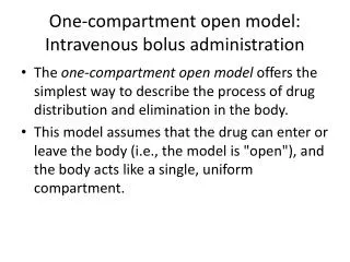
Assumptions of the model • Upon drug absorption there is instantaneous distribution of drug throughout the central compartment (sampling compartment) having a volume V1 (Vc) • Transfer of drug from the central compartment to the peripheral compartment is by a first-order process • Transfer of drug from of drug from the peripheral compartment to the central compartment is by a first-order process
Drug concentrations in the two compartments following a single i.v. bolus injection • We start with virtually no drug in the second compartment, but re-equilibration moves drug in – levels rise • A brief equilibrium - no net movement – at the peak of the curve, levels are neither rising nor falling • Re-equilibration moves into reverse and drug leaves the second compartment – levels fall
X1 X2 K12 K21 K10 Distribution rate from X1 to X2 = Distribution rate from X2 to X1 = Elimination rate =
Amount in the central compartment Conc in the central compartment VC is the volume of the central compartment Amount in the peripheral compartment
Determination of the postdistributionrate constant (β) and thecoefficient (B) • Postdistribution phase to determine: • Determine β from the graph by using the slope • The y-axis intercept of the extrapolated line is B
Determination of thedistribution rate constant (α) andthe coefficient (A) • Method of residuals: The difference between measured concentrations and those obtained by extrapolation of the post-distribution line is plotted vs time • Determine α from the graph by using the slope • The y-axis intercept of the extrapolated line is A
Determination of micro rate constants: the inter-compartmental rate constants (K21 and K12) and the pure elimination rate constant (K10)
Volume of distribution of the central compartment (VC) • Volume of distribution of the central compartment (VC). This is a proportionality constant that relates the amount of drug and the plasma concentration immediately (i.e. at t=0) following the administration of a drug.
Volume of distribution during the terminal phase (Vb or Vβ) • This is a proportionality constant that relates the plasma concentration and the amount of drug remaining in the body at a time following the attainment of distribution equilibrium, or at a time on the terminal linear portion of the plasma concentration time data
Volume of distribution at steady state (Vss) • This is a proportionality constant that relates the plasma concentration and the amount of drug remaining in the body at a time, following the attainment of practical steady state. This volume of distribution is independent of elimination parameters such as K10 or drug clearance.
The area under the plasmaconcentrationtime curve (AUC) • Model independent: Trapezoid method • Model dependent:
Example: The pharmacokinetics of amrinone after a single IV bolus injection (75 mg) in 14 healthy adult male volunteers followed a two-compartment open model and fit the following parameters: A = 4.62 ± 12.0 µg/mL B = 0.64 ± 0.17 µg/mL = 8.94 ± 13 hr–1 = 0.19 ± 0.06 hr–1 From these data, calculate: a. The volume of the central compartment b. The volume of the tissue compartment c. The transfer constants k12 and k21 d. The elimination rate constant from the central compartment e. The elimination half-life of amrinone after the drug has equilibrated with the tissue compartment
Two Compartment Extravascular Xa X1 X2 Ka K12 K21 K10
Two Compartment Extravascular Xa X1 X2 Ka K12 K21 K10