Download
1 / 1
10 likes | 108 Vues
SST Anomalies of ENSO and the Madden-Julian Oscillation: A Study with NCEP Global Ocean Data Assimilation System Yan Xue and Kyong-Hwan Seo Climate Prediction Center/NCEP/NOAA, yan.xue@noaa.gov, Kyong-Hwan.Seo@noaa.gov. CDWS2004: P4.11. INTRODUCTION

E N D
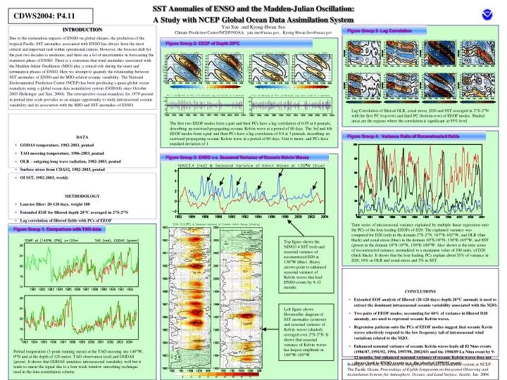
SST Anomalies of ENSO and the Madden-Julian Oscillation: A Study with NCEP Global Ocean Data Assimilation System Yan Xue and Kyong-Hwan Seo Climate Prediction Center/NCEP/NOAA, yan.xue@noaa.gov, Kyong-Hwan.Seo@noaa.gov CDWS2004: P4.11 INTRODUCTION Due to the tremendous impacts of ENSO on global climate, the prediction of the tropical Pacific SST anomalies associated with ENSO has always been the most critical and important task within operational centers. However, the forecast skill for the past two decades is moderate, and there are a lot of uncertainties in forecasting the transition phase of ENSO. There is a consensus that wind anomalies associated with the Madden-Julian Oscillation (MJO) play a critical role during the onset and termination phases of ENSO. Here we attempt to quantify the relationship between SST anomalies of ENSO and the MJO-related oceanic variability. The National Environmental Prediction Center (NCEP) has been producing a quasi-global ocean reanalysis using a global ocean data assimilation system (GODAS) since October 2003 (Behringer and Xue, 2004). The retrospective ocean reanalysis for 1979-present in pentad time scale provides us an unique opportunity to study intraseasonal oceanic variability and its association with the MJO and SST anomalies of ENSO. Figure Group 3: Lag Correlation Figure Group 2: EEOF of Depth 20OC Lag Correlation of filtered OLR, zonal stress, D20 and SST averaged in 2OS-2ON with the first PC (top row) and third PC (bottom row) of EEOF modes. Shaded areas are the regions where the correlation is significant at 95% level. • DATA • GODAS temperature, 1982-2003, pentad • TAO mooring temperature, 1986-2003, pentad • OLR – outgoing long wave radiation, 1982-2003, pentad • Surface stress from CDAS2, 1982-2003, pentad • OI SST, 1982-2003, weekly The first two EEOF modes form a pair and their PCs have a lag correlation of 0.95 at 4 pentads, describing an eastward propagating oceanic Kelvin wave at a period of 80 days. The 3rd and 4th EEOF modes form a pair and their PCs have a lag correlation of 0.9 at 3 pentads, describing an eastward propagating oceanic Kelvin wave at a period of 60 days. Unit is meter, and PCs have standard deviation of 1. Figure Group 4: Variance Ratio of Reconstructed fields Figure Group 5: ENSO v.s. Seasonal Variance of Oceanic Kelvin Waves • METHODOLOGY • Lanczos filter: 20-120 days, weight 100 • Extended EOF for filtered depth 20OC averaged in 2OS-2ON • Lag correlation of filtered fields with PCs of EEOF • Reconstruction using regression patterns onto the first two pairs of PCs Time series of intraseasonal variance explained by multiple linear regression onto the PCs of the four leading EEOFs of D20. The explained variance was computed for D20 (red) in the domain 2OS-2ON, 167OE-102OW, and OLR (thin black) and zonal stress (blue) in the domain 10OS-10ON, 130OE-165OW, and SST (green) in the domain 10OS-10ON, 130OE-100OW. Also shown is the time series of reconstructed variance, normalized to a maximum value of 100 units, of D20 (thick black). It shows that the four leading PCs explain about 55% of variance in D20, 10% in OLR and zonal stress and 5% in SST. Figure Group 1: Comparison with TAO data Top figure shows the NINO3.4 SST (red) and seasonal variance of reconstructed D20 at 130OW (blue). Heavy arrows point to enhanced seasonal variance of Kelvin waves that lead ENSO events by 9-12 months. • CONCLUSIONS • Extended EOF analysis of filtered (20-120 days) depth 20OC anomaly is used to extract the dominant intraseasonal oceanic variability associated with the MJO. • Two pairs of EEOF modes, accounting for 60% of variance in filtered D20 anomaly, are used to represent oceanic Kelvin waves. • Regression patterns onto the PCs of EEOF modes suggest that oceanic Kevin waves selectively respond to the low frequency tail of intraseasonal wind variations related to the MJO. • Enhanced seasonal variance of oceanic Kelvin waves leads all El Nino events (1986/87, 1991/92, 1994, 1997/98, 2002/03) and the 1988/89 La Nina event by 9-12 months, but enhanced seasonal variance of oceanic Kelvin waves does not always lead to ENSO events (e.g. the aborted 1990/91 event). Left figure shows Hovmoeller diagram of SST anomalies (contour) and seasonal variance of Kelvin waves (shaded) averaged over 2OS-2ON. It shows that seasonal variance of Kelvin waves has largest amplitude in 180OW-105OW. Pentad temperature (3-point-running mean) at the TAO mooring site 140OW, 0ON and at the depth of 120 meter. TAO observation (red) and GODAS (green). It shows that GODAS simulates intraseasonal variability well but it tends to smear the signal due to a four week window smoothing technique used in the data assimilation scheme. Behringer and Xue, Evaluation of the global ocean data assimilation system at NCEP: The Pacific Ocean.Proceedings of Eighth Symposium on Integrated Observing and Assimilation Systems for Atmosphere, Oceans, and Land Surface, Seattle,Jan. 2004.